Large dataset with 500 patients for testing computational efficiency and performance with substantial sample sizes. Three tests with good characteristics.
Format
A data frame with 500 rows and 7 variables:
- patient_id
Character: Patient identifier (PT0001-PT0500)
- Test1
Factor: First test ("Negative", "Positive"), Sens=0.87, Spec=0.87
- Test2
Factor: Second test ("Negative", "Positive"), Sens=0.84, Spec=0.89
- Test3
Factor: Third test ("Negative", "Positive"), Sens=0.81, Spec=0.91
- age
Numeric: Patient age in years (mean 59, SD 13)
- sex
Factor: "Male" or "Female"
- study_center
Factor: Multi-center study (Center_1 to Center_8)
Details
Simulated with 28% prevalence. Large sample (n=500) from multi-center study tests computational efficiency and precision of estimates.
Examples
data(nogoldstandard_large)
nogoldstandard(data = nogoldstandard_large,
               test1 = "Test1", test1Positive = "Positive",
               test2 = "Test2", test2Positive = "Positive",
               test3 = "Test3", test3Positive = "Positive",
               test4Positive = "", test5Positive = "")
#>
#>  ANALYSIS WITHOUT GOLD STANDARD
#> Analysing 500 cases
#> All 500 cases have a result for every selected test.
#>  Agreement Statistics (Cohen's Kappa)
#>  ──────────────────────────────────────────────────────────
#>    Test Pair         Kappa        p-value       Agreement
#>  ──────────────────────────────────────────────────────────
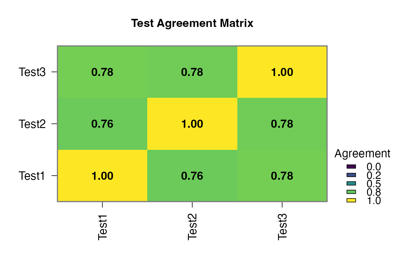
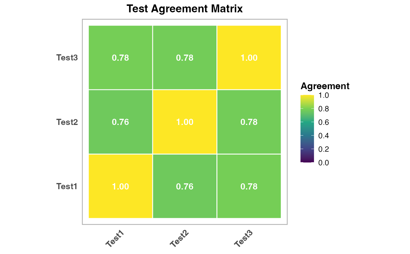
#>    Test1 vs Test2    0.4502935    < .0000001     76.40000
#>    Test1 vs Test3    0.4880061    < .0000001     78.40000
#>    Test2 vs Test3    0.4669205    < .0000001     77.60000
#>  ──────────────────────────────────────────────────────────
#>    Note. Kappa standard errors and p-values use a
#>    large-sample normal approximation rather than the
#>    exact asymptotic SE (e.g. vcd::Kappa); interpret
#>    p-values cautiously, especially in small samples.
#>
#>
#>  <div class='clinical-summary' style='background: #f0f8ff; padding:
#>  15px; border-radius: 8px; margin: 10px 0;'><h4 style='color: #1565c0;
#>  margin-top: 0;'> Clinical Summary
#>
#>  Analysis: No gold standard analysis using latent_class method
#>
#>  Tests analyzed: Test1, Test2, Test3 (N=3)
#>
#>  Disease prevalence: 27.8%
#>
#>  Test sensitivities: Range from 80.0% to 82.8%
#>
#>  Clinical interpretation: Moderate prevalence setting - balanced
#>  diagnostic performance
#>
#>  <div style='background: #f8f9fa; padding: 20px; border-radius: 8px;
#>  margin: 15px 0; border-left: 4px solid #007bff;'><h3 style='color:
#>  #007bff; margin-top: 0;'> Method Selection Guide
#>
#>  <div style='margin: 15px 0; padding: 15px; background: #e8f5e8;
#>  border-radius: 5px;'><h4 style='color: #2e7d32; margin-top: 0;'>
#>  Latent Class Analysis (Recommended)
#>
#>  Description: Most robust method using mixture models. Estimates
#>  disease prevalence and test parameters simultaneously.
#>
#>  Best for: Diagnostic validation studies with 3+ tests and N>=100
#>
#>  Strengths: The only method here that estimates accuracy rather than
#>  agreement with a self-built reference; provides model fit statistics.
#>  Assumes the tests are conditionally independent given true status --
#>  it does NOT model conditional dependence
#>
#>  <div style='margin: 15px 0; padding: 15px; background: #e3f2fd;
#>  border-radius: 5px;'><h4 style='color: #1565c0; margin-top: 0;'>
#>  Bayesian Analysis
#>
#>  Description: Incorporates prior knowledge about test performance using
#>  Bayesian methods.
#>
#>  Best for: Studies where you have prior information about expected
#>  sensitivity/specificity
#>
#>  Strengths: Uses prior knowledge, handles uncertainty well, good for
#>  smaller samples
#>
#>  <div style='margin: 15px 0; padding: 15px; background: #fff3e0;
#>  border-radius: 5px;'><h4 style='color: #ef6c00; margin-top: 0;'>
#>  Composite Reference
#>
#>  Description: Uses majority vote of available tests as pseudo-gold
#>  standard.
#>
#>  Best for: Inter-rater agreement studies with 3+ tests, exploratory
#>  analysis
#>
#>  Strengths: Simple and intuitive. Not an accuracy estimate: each test
#>  helps build the standard it is judged against, which inflates its
#>  apparent performance. Needs 3+ tests -- with 2 a tie counts as
#>  diseased, making it identical to Any Test Positive
#>
#>  <div style='margin: 15px 0; padding: 15px; background: #fce4ec;
#>  border-radius: 5px;'><h4 style='color: #c2185b; margin-top: 0;'> All
#>  Tests Positive
#>
#>  Description: Conservative approach - disease present only if ALL tests
#>  are positive.
#>
#>  Best for: Highly specific diagnoses where false positives are very
#>  costly
#>
#>  Strengths: A deliberately strict reference. Sensitivity and NPV cannot
#>  be estimated under this rule -- they are fixed at 100% by construction
#>  -- so only specificity and PPV are shown, and both are inflated by the
#>  same circularity
#>
#>  <div style='margin: 15px 0; padding: 15px; background: #e8f5e8;
#>  border-radius: 5px;'><h4 style='color: #388e3c; margin-top: 0;'> Any
#>  Test Positive
#>
#>  Description: Liberal approach - disease present if ANY test is
#>  positive.
#>
#>  Best for: Population screening scenarios where missing cases is costly
#>
#>  Strengths: A deliberately permissive reference. Specificity and PPV
#>  cannot be estimated under this rule -- they are fixed at 100% by
#>  construction -- so only sensitivity and NPV are shown, and both are
#>  inflated by the same circularity
#>
#>  <div style='margin: 15px 0; padding: 10px; background: #fff8e1;
#>  border-radius: 5px; border-left: 3px solid #ffb300;'><h4 style='color:
#>  #e65100; margin-top: 0;'> Selection Tips
#>
#>  Start with Latent Class Analysis for most diagnostic studiesUse
#>  Composite Reference for quick exploratory analysisChoose All/Any Tests
#>  Positive based on clinical consequences of errorsConsider Bayesian if
#>  you have strong prior information
#>
#>  Disease Prevalence
#>  ───────────────────────────────────────
#>    Estimate     Lower CI     Upper CI
#>  ───────────────────────────────────────
#>     27.76421     23.83883     31.68959
#>  ───────────────────────────────────────
#>
#>
#>  Test Performance Metrics
#>  ─────────────────────────────────────────────────────────────────────────────────────────────────────────────────────
#>    Test     Sensitivity    Lower CI     Upper CI     Specificity    Lower CI     Upper CI     PPV          NPV
#>  ─────────────────────────────────────────────────────────────────────────────────────────────────────────────────────
#>    Test1       82.77059     76.48865     89.05253       88.34456     85.03522     91.65390     73.18662     93.02681
#>    Test2       79.95526     73.29572     86.61480       87.81621     84.44283     91.18960     71.60950     91.93440
#>    Test3       81.13588     74.62792     87.64385       91.03870     88.09302     93.98438     77.67840     92.62328
#>  ─────────────────────────────────────────────────────────────────────────────────────────────────────────────────────
#>    Note. 95% intervals are normal-approximation (Wald) intervals, using the estimated number of diseased cases as
#>    the denominator for sensitivity and non-diseased for specificity. They treat the estimates as observed
#>    proportions and so understate the uncertainty of a latent-variable model; enable Bootstrap for intervals that
#>    account for the estimation itself.
#>
#>
#>  Model Fit Statistics
#>  ─────────────────────────────────────
#>    Statistic             Value
#>  ─────────────────────────────────────
#>    BIC                   1629.938355
#>    AIC                   1600.436098
#>    Log-Likelihood        -793.218049
#>    Degrees of Freedom       0.000000
#>  ─────────────────────────────────────
#>    Note. With three tests this
#>    model has as many parameters as
#>    the data can support (0
#>    residual degrees of freedom),
#>    so it reproduces the observed
#>    table exactly. Goodness-of-fit
#>    statistics are therefore
#>    omitted: they cannot tell you
#>    whether the
#>    conditional-independence
#>    assumption holds. Use four or
#>    more tests if you need to test
#>    the model's fit.
#>
#>
#>  Conditional Independence Check (Bivariate Residuals)
#>  ─────────────────────────────────────────────────────
#>    Test Pair    Bivariate Residual    Interpretation
#>  ─────────────────────────────────────────────────────
#>  ─────────────────────────────────────────────────────
#>    Note. Not computable with three tests: the
#>    model has no residual degrees of freedom, so it
#>    reproduces every observed table exactly and no
#>    residual can detect conditional dependence. Add
#>    a fourth test if you need to check this
#>    assumption.
#>
#>
#>  Test Cross-Tabulation
#>  ─────────────────────────────────────────────────
#>    Test Combination          Count    Percentage
#>  ─────────────────────────────────────────────────
#>    Test1-, Test2-, Test3-      256      51.20000
#>    Test1+, Test2+, Test3+       75      15.00000
#>    Test1-, Test2+, Test3-       39       7.80000
#>    Test1+, Test2-, Test3-       38       7.60000
#>    Test1-, Test2-, Test3+       29       5.80000
#>    Test1+, Test2+, Test3-       22       4.40000
#>    Test1+, Test2-, Test3+       22       4.40000
#>    Test1-, Test2+, Test3+       19       3.80000
#>  ─────────────────────────────────────────────────
#>