jjscatterstats: Comprehensive Scatter Plot Analysis

Introduction to jjscatterstats

The jjscatterstats function is a powerful wrapper around ggstatsplot::ggscatterstats() and ggstatsplot::grouped_ggscatterstats() that provides comprehensive scatter plot analysis with statistical testing capabilities. This function is particularly useful for exploring relationships between continuous variables in clinical and research settings.

Key Features

Statistical Analysis: Automatic correlation analysis with multiple statistical approaches
Flexible Grouping: Support for grouped analysis across categorical variables
Multiple Statistical Types: Parametric, non-parametric, robust, and Bayesian statistics
Customizable Visualization: Extensive theming and labeling options
Performance Optimized: Enhanced caching and data preparation for faster rendering

Loading Required Libraries

library(jjstatsplot)
library(ggplot2)
library(dplyr)

# Load example datasets
data(iris)
data(mtcars)

Basic Scatter Plot Analysis

Simple Correlation Analysis

Let’s start with a basic scatter plot analyzing the relationship between sepal length and petal length in the iris dataset:

# Basic scatter plot with parametric correlation
result_basic <- jjscatterstats(
  data = iris,
  dep = "Sepal.Length",
  group = "Petal.Length",
  typestatistics = "parametric",
  mytitle = "Sepal Length vs Petal Length",
  xtitle = "Sepal Length (cm)",
  ytitle = "Petal Length (cm)"
)

print(result_basic)
#> 
#>  SCATTER PLOT
#> 
#>  You have selected to use a scatter plot with correlation analysis.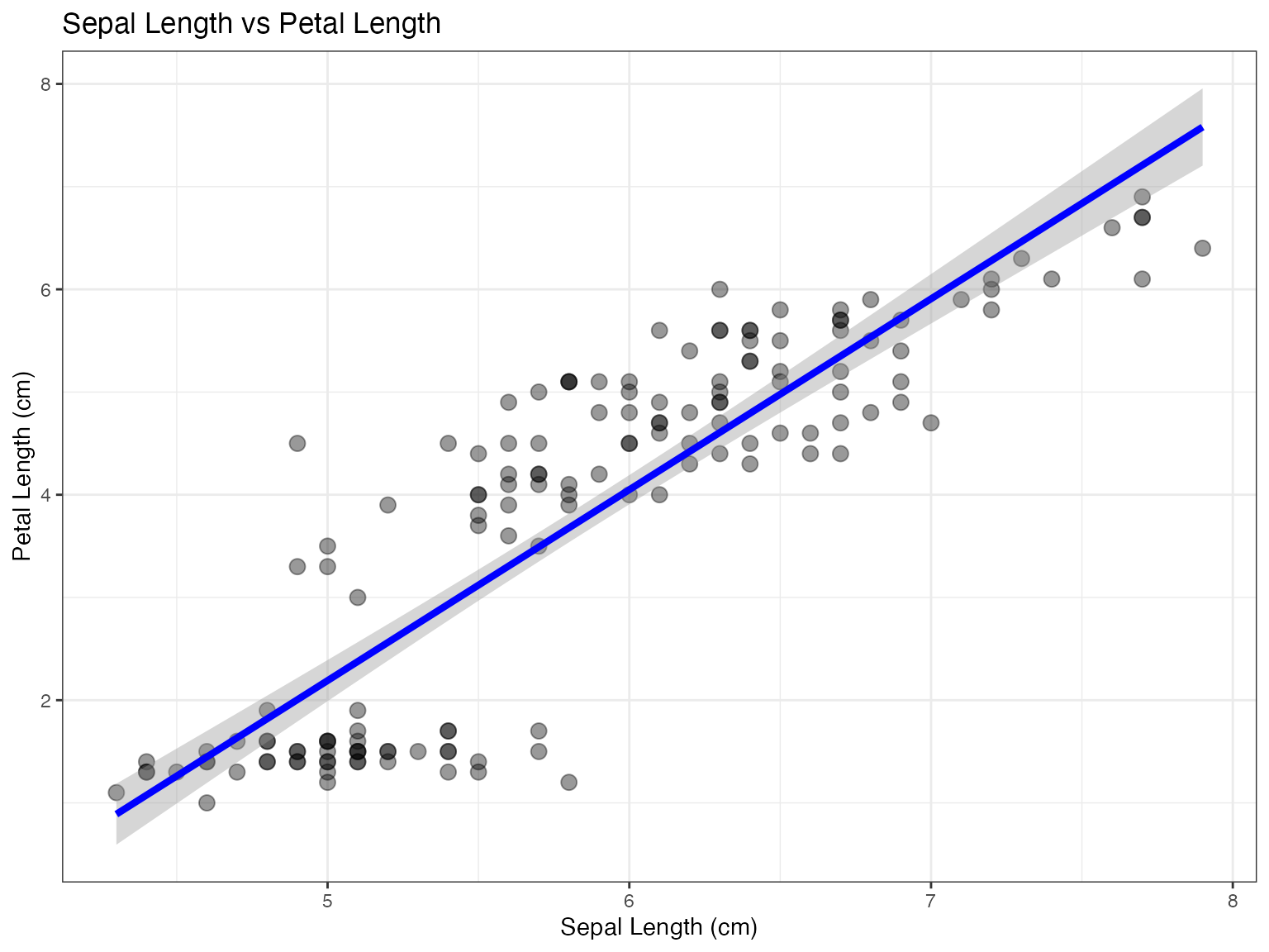

Different Statistical Approaches

Non-parametric Analysis

# Non-parametric correlation (Spearman's rho)
result_nonparam <- jjscatterstats(
  data = iris,
  dep = "Sepal.Length",
  group = "Petal.Width",
  typestatistics = "nonparametric",
  mytitle = "Non-parametric Correlation Analysis"
)

print(result_nonparam)
#> 
#>  SCATTER PLOT
#> 
#>  You have selected to use a scatter plot with correlation analysis.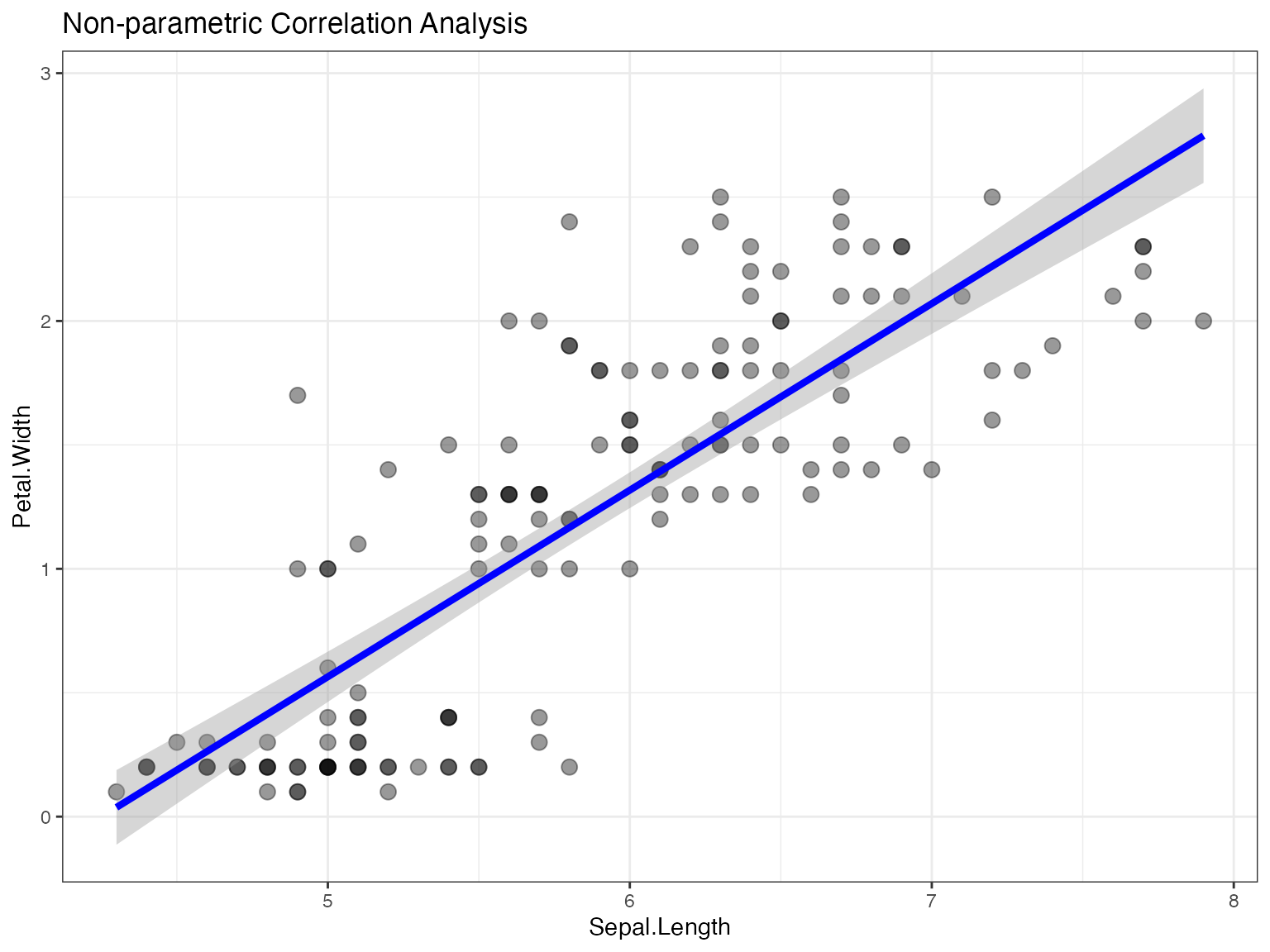

Robust Statistics

# Robust correlation analysis
result_robust <- jjscatterstats(
  data = iris,
  dep = "Sepal.Width",
  group = "Petal.Length",
  typestatistics = "robust",
  mytitle = "Robust Correlation Analysis"
)

print(result_robust)
#> 
#>  SCATTER PLOT
#> 
#>  You have selected to use a scatter plot with correlation analysis.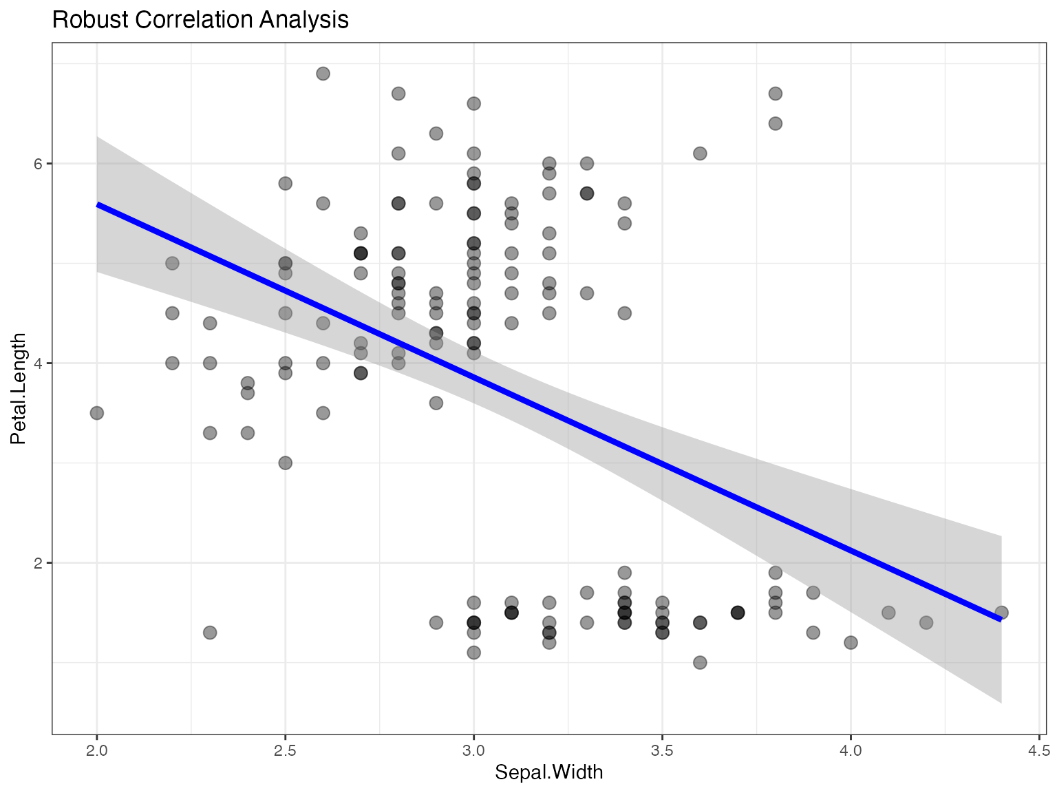

Bayesian Analysis

# Bayesian correlation analysis
result_bayes <- jjscatterstats(
  data = iris,
  dep = "Sepal.Length",
  group = "Sepal.Width",
  typestatistics = "bayes",
  mytitle = "Bayesian Correlation Analysis"
)

print(result_bayes)
#> 
#>  SCATTER PLOT
#> 
#>  You have selected to use a scatter plot with correlation analysis.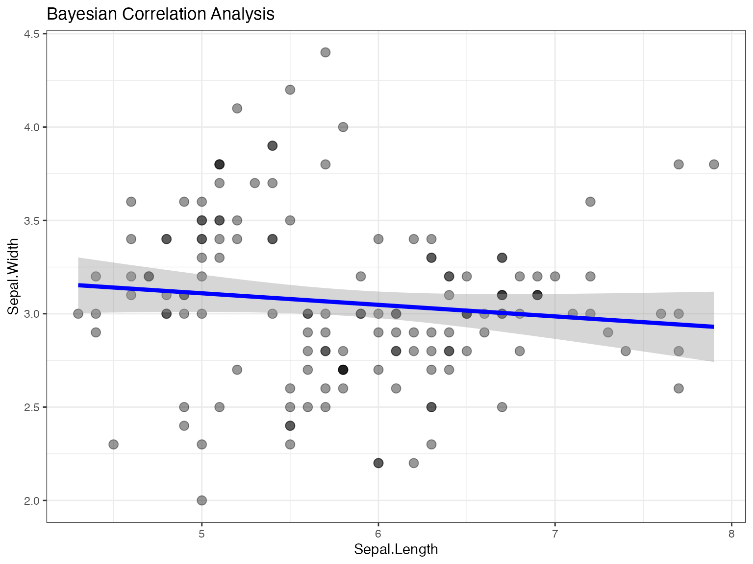

Grouped Analysis

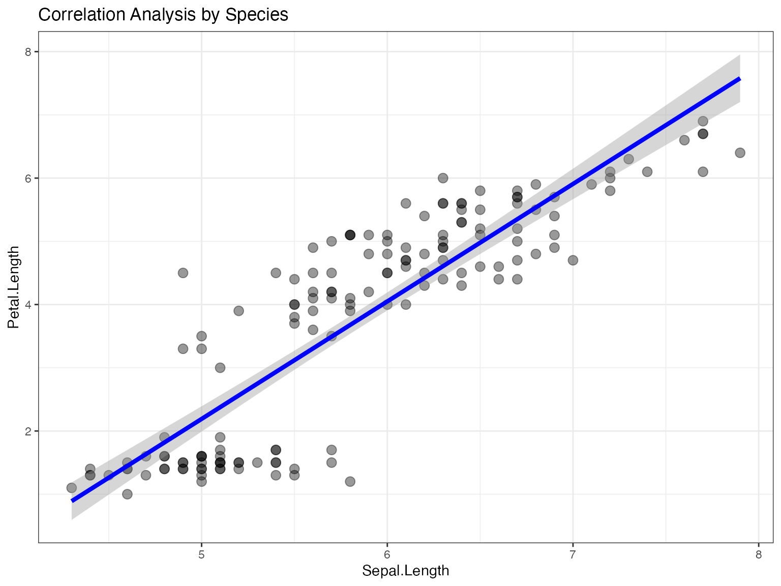
Scatter Plot by Species

One of the most powerful features is the ability to create grouped scatter plots:

# Grouped scatter plot by species
result_grouped <- jjscatterstats(
  data = iris,
  dep = "Sepal.Length",
  group = "Petal.Length",
  grvar = "Species",
  typestatistics = "parametric",
  mytitle = "Correlation Analysis by Species"
)

print(result_grouped)
#> 
#>  SCATTER PLOT
#> 
#>  You have selected to use a scatter plot with correlation analysis.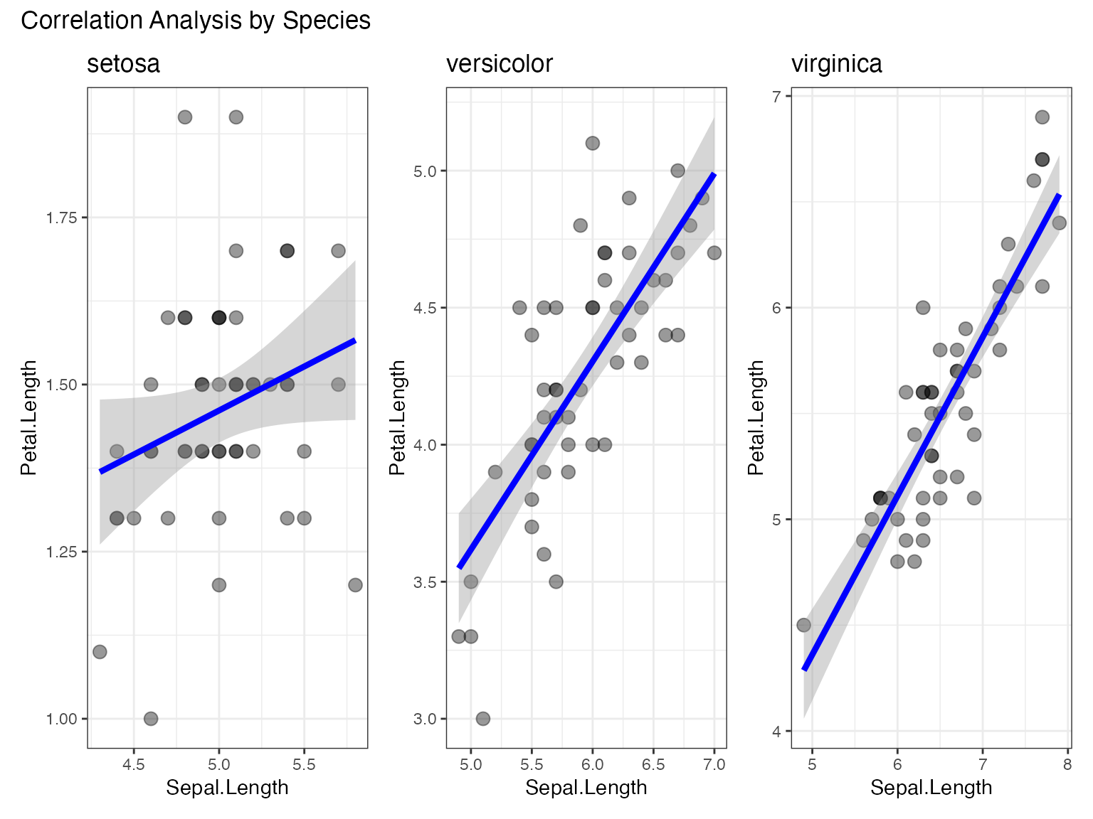

Multiple Group Analysis with mtcars

# Prepare mtcars data
mtcars_modified <- mtcars %>%
  mutate(
    transmission = factor(am, levels = c(0, 1), labels = c("Automatic", "Manual")),
    cylinders = factor(cyl)
  )

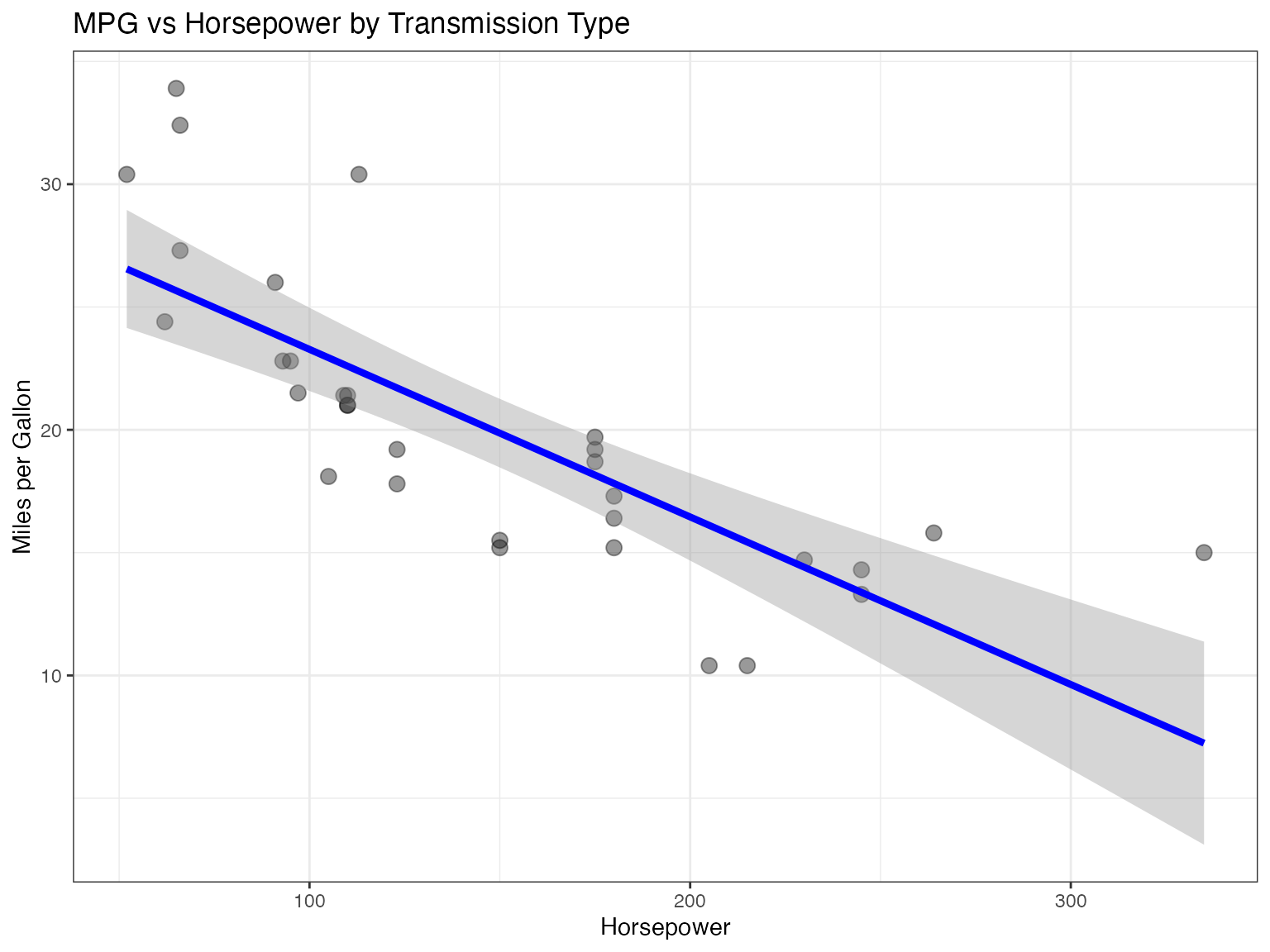
# Grouped analysis of mpg vs horsepower by transmission type
result_mtcars <- jjscatterstats(
  data = mtcars_modified,
  dep = "hp",
  group = "mpg",
  grvar = "transmission",
  typestatistics = "parametric",
  mytitle = "MPG vs Horsepower by Transmission Type",
  xtitle = "Horsepower",
  ytitle = "Miles per Gallon"
)

print(result_mtcars)
#> 
#>  SCATTER PLOT
#> 
#>  You have selected to use a scatter plot with correlation analysis.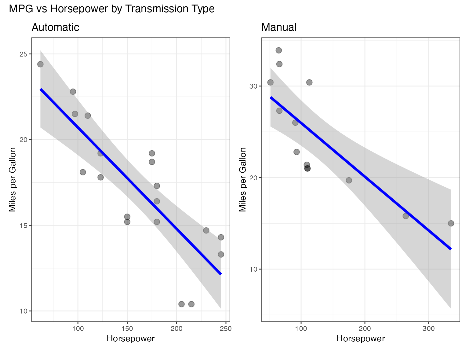

Clinical Research Applications

Using Clinical Test Data

# Example with clinical data (if available)
# This demonstrates typical clinical research scenarios

# Load clinical test data
data(jjscatterstats_clinical)

# Analyze tumor size vs Ki67 percentage
clinical_result <- jjscatterstats(
  data = jjscatterstats_clinical,
  dep = "tumor_size_mm",
  group = "ki67_percentage",
  grvar = "stage",
  typestatistics = "parametric",
  mytitle = "Tumor Size vs Ki67 by Cancer Stage",
  xtitle = "Tumor Size (mm)",
  ytitle = "Ki67 Percentage (%)"
)

print(clinical_result)

Biomarker Correlation Analysis

# Biomarker correlation analysis
biomarker_result <- jjscatterstats(
  data = jjscatterstats_clinical,
  dep = "mutation_count",
  group = "survival_months",
  grvar = "histology",
  typestatistics = "nonparametric",
  mytitle = "Mutation Count vs Survival by Histology",
  xtitle = "Mutation Count",
  ytitle = "Survival (months)"
)

print(biomarker_result)

Advanced Customization

Theme Customization

# Using original ggstatsplot theme
result_original_theme <- jjscatterstats(
  data = iris,
  dep = "Sepal.Length",
  group = "Petal.Length",
  originaltheme = TRUE,
  mytitle = "Original ggstatsplot Theme"
)

print(result_original_theme)
#> 
#>  SCATTER PLOT
#> 
#>  You have selected to use a scatter plot with correlation analysis.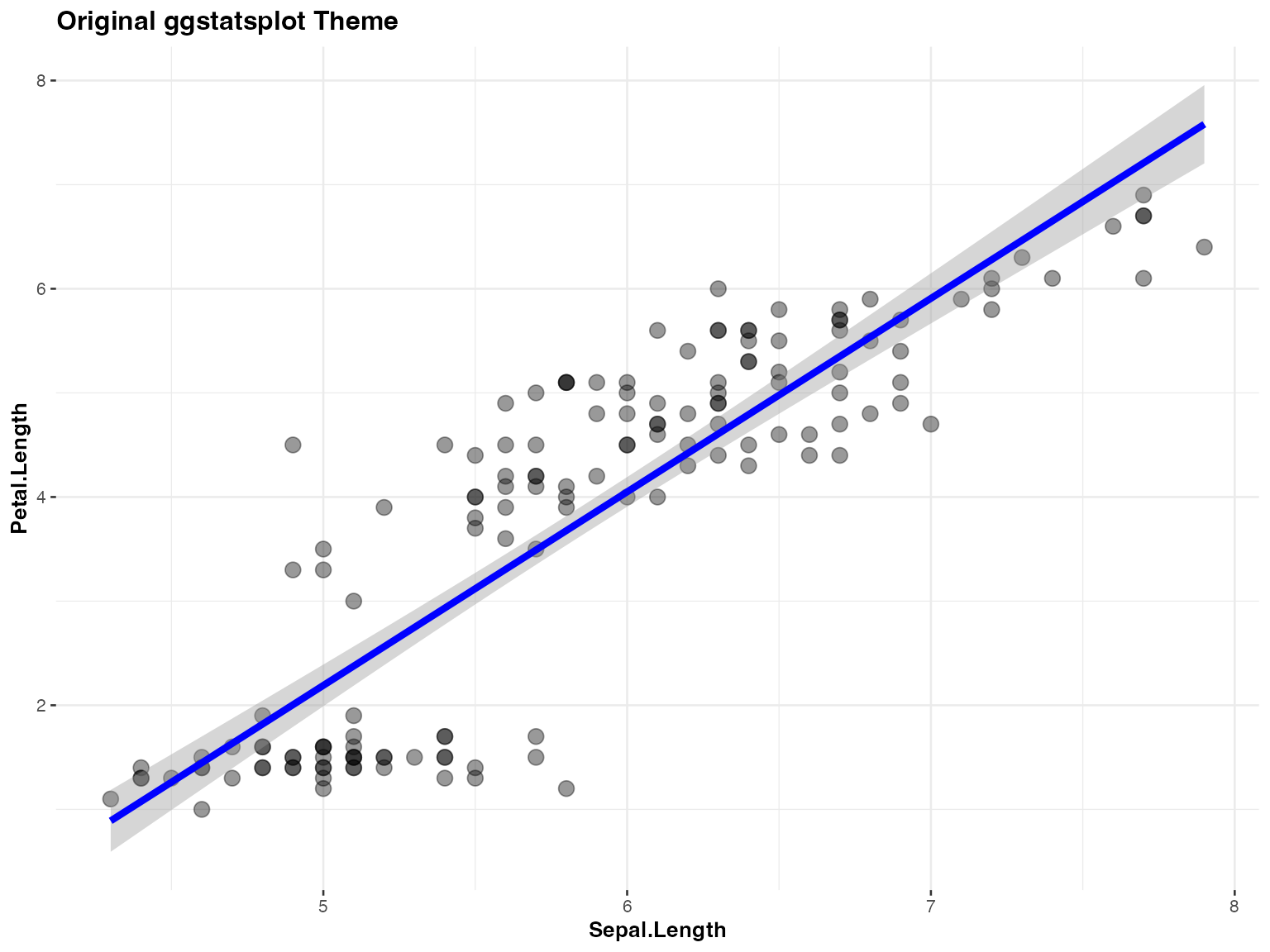

Custom Labels and Titles

# Comprehensive labeling
result_labeled <- jjscatterstats(
  data = mtcars,
  dep = "wt",
  group = "mpg",
  typestatistics = "parametric",
  mytitle = "Vehicle Weight vs Fuel Efficiency",
  xtitle = "Weight (1000 lbs)",
  ytitle = "Miles per Gallon",
  resultssubtitle = TRUE
)

print(result_labeled)
#> 
#>  SCATTER PLOT
#> 
#>  You have selected to use a scatter plot with correlation analysis.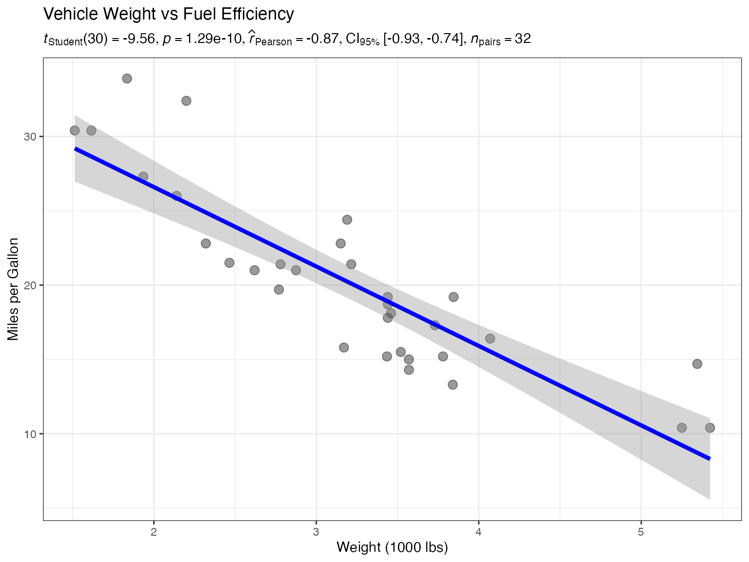

Controlling Statistical Results Display

# Hide statistical results subtitle
result_no_stats <- jjscatterstats(
  data = iris,
  dep = "Sepal.Width",
  group = "Petal.Width",
  typestatistics = "parametric",
  mytitle = "Clean Plot Without Statistics",
  resultssubtitle = FALSE
)

print(result_no_stats)
#> 
#>  SCATTER PLOT
#> 
#>  You have selected to use a scatter plot with correlation analysis.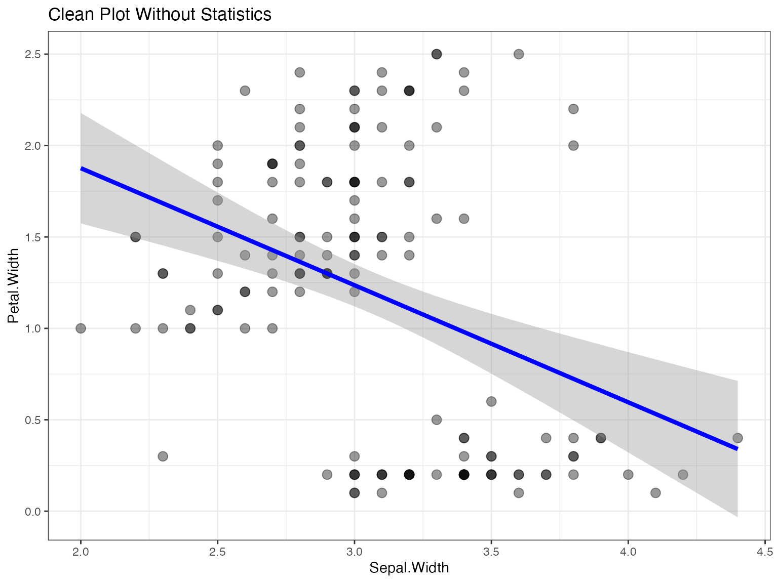

Performance Considerations

Large Dataset Handling

The function includes several performance optimizations:

# Performance test with larger dataset
data(jjscatterstats_performance)

# This should render efficiently due to optimizations
start_time <- Sys.time()
performance_result <- jjscatterstats(
  data = jjscatterstats_performance,
  dep = "measurement_1",
  group = "measurement_2",
  grvar = "lab_id",
  typestatistics = "parametric",
  mytitle = "Performance Test - Large Dataset"
)
end_time <- Sys.time()

cat("Rendering time:", difftime(end_time, start_time, units = "secs"), "seconds\n")
print(performance_result)

Data Caching and Optimization

The function implements several performance enhancements:

Data Preparation Caching: Processed data is cached to avoid recomputation
Option Preprocessing: Common option processing is done once and cached
Hash-based Change Detection: Only reprocesses data when inputs change
Efficient Memory Usage: Minimizes data copying and transformation overhead

Edge Cases and Data Validation

Handling Missing Values

# Create data with missing values
iris_with_na <- iris
iris_with_na[1:10, "Sepal.Length"] <- NA
iris_with_na[15:20, "Petal.Length"] <- NA

# Function automatically handles missing values
result_na <- jjscatterstats(
  data = iris_with_na,
  dep = "Sepal.Length",
  group = "Petal.Length",
  typestatistics = "parametric",
  mytitle = "Handling Missing Values"
)

print(result_na)
#> 
#>  SCATTER PLOT
#> 
#>  You have selected to use a scatter plot with correlation analysis.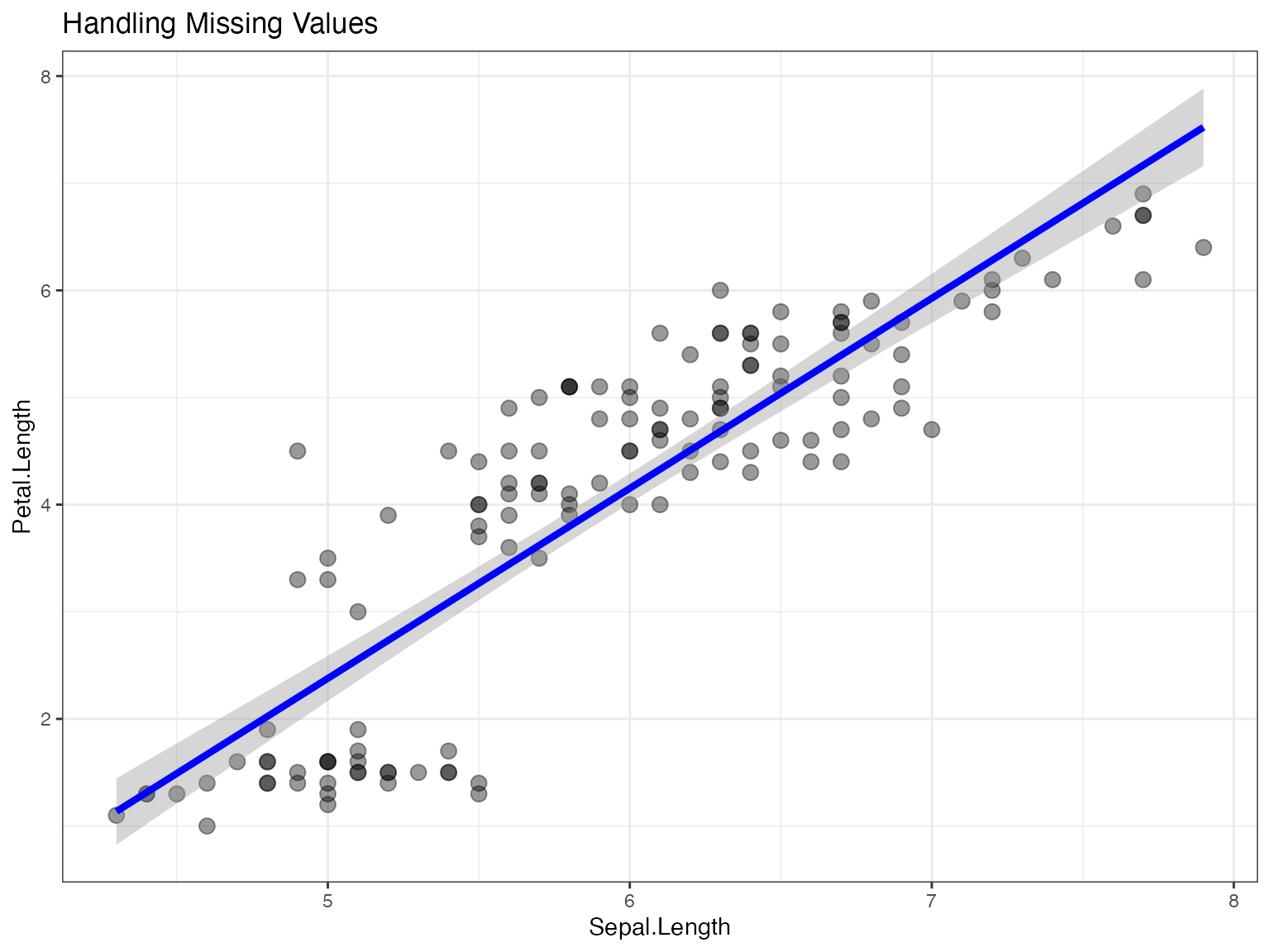

Input Validation

# Example of error handling
try({
  result_error <- jjscatterstats(
    data = data.frame(),  # Empty dataset
    dep = "nonexistent",
    group = "variable",
    typestatistics = "parametric"
  )
})
#> Error : Argument 'dep' contains 'nonexistent' which is not present in the dataset

Best Practices and Recommendations

Statistical Type Selection

Parametric: Use when data is normally distributed (Pearson correlation)
Non-parametric: Use for non-normal data or ordinal variables (Spearman correlation)
Robust: Use when data has outliers (percentage bend correlation)
Bayesian: Use for incorporating prior knowledge or uncertainty quantification

Visualization Guidelines

Choose appropriate variables: Both x and y should be continuous
Consider grouping: Use grouping variables to reveal subgroup patterns
Label clearly: Always provide meaningful titles and axis labels
Statistical reporting: Include statistical results unless specifically hiding them

Performance Tips

Large datasets: The function is optimized for datasets up to several thousand rows
Multiple analyses: Reuse data objects when possible to benefit from caching
Grouping variables: Limit grouping variables to reasonable numbers of levels (< 10)

Troubleshooting Common Issues

Variable Type Issues

# Ensure variables are numeric
str(iris[c("Sepal.Length", "Petal.Length")])
#> 'data.frame':    150 obs. of  2 variables:
#>  $ Sepal.Length: num  5.1 4.9 4.7 4.6 5 5.4 4.6 5 4.4 4.9 ...
#>  $ Petal.Length: num  1.4 1.4 1.3 1.5 1.4 1.7 1.4 1.5 1.4 1.5 ...

# The function automatically converts to numeric, but it's good practice to check

Memory and Performance

# For very large datasets, consider:
# 1. Sampling your data first
set.seed(123)
sampled_data <- iris[sample(nrow(iris), 100), ]

result_sampled <- jjscatterstats(
  data = sampled_data,
  dep = "Sepal.Length",
  group = "Petal.Length",
  typestatistics = "parametric"
)

# 2. Using simpler statistical methods for initial exploration
result_simple <- jjscatterstats(
  data = iris,
  dep = "Sepal.Length",
  group = "Petal.Length",
  typestatistics = "parametric",
  resultssubtitle = FALSE  # Faster rendering
)

Summary

The jjscatterstats function provides a comprehensive solution for scatter plot analysis with:

Multiple statistical testing approaches
Flexible grouping capabilities
Performance optimizations for larger datasets
Extensive customization options
Robust error handling and validation

This makes it an excellent choice for exploratory data analysis, clinical research, and statistical reporting in the jamovi environment.

Function Reference

For complete parameter documentation, see:

# Session information
sessionInfo()
#> R version 4.6.0 (2026-04-24)
#> Platform: aarch64-apple-darwin23
#> Running under: macOS Tahoe 26.5.2
#> 
#> Matrix products: default
#> BLAS:   /Library/Frameworks/R.framework/Versions/4.6/Resources/lib/libRblas.0.dylib 
#> LAPACK: /Library/Frameworks/R.framework/Versions/4.6/Resources/lib/libRlapack.dylib;  LAPACK version 3.12.1
#> 
#> locale:
#> [1] en_US.UTF-8/en_US.UTF-8/en_US.UTF-8/C/en_US.UTF-8/en_US.UTF-8
#> 
#> time zone: Europe/Istanbul
#> tzcode source: internal
#> 
#> attached base packages:
#> [1] stats     graphics  grDevices utils     datasets  methods   base     
#> 
#> other attached packages:
#> [1] dplyr_1.2.1           ggplot2_4.0.3         jjstatsplot_1.0.53.01
#> 
#> loaded via a namespace (and not attached):
#>   [1] ggstatsplot_1.0.0         splines_4.6.0            
#>   [3] later_1.4.8               tibble_3.3.1             
#>   [5] ggpp_0.6.1                jmvcore_2.7.38           
#>   [7] polyclip_1.10-7           datawizard_1.3.1         
#>   [9] hardhat_1.4.3             rpart_4.1.27             
#>  [11] ggExtra_0.11.0            lifecycle_1.0.5          
#>  [13] rstatix_1.1.0             globals_0.19.1           
#>  [15] lattice_0.22-9            MASS_7.3-66              
#>  [17] insight_1.5.2             ggdist_3.3.3             
#>  [19] backports_1.5.1           magrittr_2.0.5           
#>  [21] sass_0.4.10               rmarkdown_2.31           
#>  [23] jquerylib_0.1.4           yaml_2.3.12              
#>  [25] httpuv_1.6.17             otel_0.2.0               
#>  [27] cowplot_1.2.0             pbapply_1.7-4            
#>  [29] RColorBrewer_1.1-3        easyalluvial_0.4.1       
#>  [31] lubridate_1.9.5           multcomp_1.4-31          
#>  [33] abind_1.4-8               purrr_1.2.2              
#>  [35] nnet_7.3-21               TH.data_1.1-5            
#>  [37] tweenr_2.0.3              sandwich_3.1-3           
#>  [39] ipred_0.9-15              lava_1.9.2               
#>  [41] ggrepel_0.9.8             listenv_1.0.0            
#>  [43] correlation_0.8.8         moments_0.14.1           
#>  [45] MatrixModels_0.5-4        parallelly_1.48.0        
#>  [47] pkgdown_2.2.1             codetools_0.2-20         
#>  [49] DT_0.34.0                 ggforce_0.5.0            
#>  [51] tidyselect_1.2.1          farver_2.1.2             
#>  [53] viridis_0.6.5             effectsize_1.0.3         
#>  [55] WRS2_1.1-7                jsonlite_2.0.0           
#>  [57] progressr_1.0.0           Formula_1.2-6            
#>  [59] ggridges_0.5.7            ggalluvial_0.12.6        
#>  [61] survival_3.8-9            emmeans_2.0.4            
#>  [63] systemfonts_1.3.2         tools_4.6.0              
#>  [65] waffle_1.0.2              ragg_1.5.2               
#>  [67] Rcpp_1.1.2                glue_1.8.1               
#>  [69] prodlim_2026.03.11        gridExtra_2.3.1          
#>  [71] Rttf2pt1_1.3.14           xfun_0.60                
#>  [73] mgcv_1.9-4                distributional_0.8.1     
#>  [75] ggsegmentedtotalbar_0.1.0 withr_3.0.3              
#>  [77] fastmap_1.2.0             boot_1.3-32              
#>  [79] digest_0.6.39             timechange_0.4.0         
#>  [81] R6_2.6.1                  mime_0.13                
#>  [83] estimability_2.0.0        ggprism_1.0.7            
#>  [85] textshaping_1.0.5         ggrain_0.1.2             
#>  [87] tidyr_1.3.2               generics_0.1.4           
#>  [89] data.table_1.18.4         recipes_1.3.3            
#>  [91] class_7.3-24              htmlwidgets_1.6.4        
#>  [93] parameters_0.29.2         pkgconfig_2.0.3          
#>  [95] gtable_0.3.6              timeDate_4052.112        
#>  [97] statsExpressions_2.0.0    S7_0.2.2                 
#>  [99] BayesFactor_0.9.12-4.8    htmltools_0.5.9          
#> [101] carData_3.0-6             scales_1.4.0             
#> [103] gower_1.0.2               knitr_1.51               
#> [105] coda_0.19-4.1             nlme_3.1-170             
#> [107] curl_7.1.0                cachem_1.1.0             
#> [109] zoo_1.9-0                 stringr_1.6.0            
#> [111] parallel_4.6.0            miniUI_0.1.2             
#> [113] extrafont_0.20            desc_1.4.3               
#> [115] pillar_1.11.1             grid_4.6.0               
#> [117] reshape_0.8.10            vctrs_0.7.3              
#> [119] promises_1.5.0            ggpubr_1.0.0             
#> [121] car_3.1-5                 xtable_1.8-8             
#> [123] extrafontdb_1.1           paletteer_1.7.0          
#> [125] evaluate_1.0.5            mvtnorm_1.4-2            
#> [127] cli_3.6.6                 compiler_4.6.0           
#> [129] rlang_1.3.0               rstantools_2.7.0         
#> [131] future.apply_1.20.2       ggsignif_0.6.4           
#> [133] labeling_0.4.3            rematch2_2.1.2           
#> [135] plyr_1.8.9                forcats_1.0.1            
#> [137] fs_2.1.0                  stringi_1.8.9            
#> [139] viridisLite_0.4.3         bayestestR_0.18.1        
#> [141] Matrix_1.7-6              hms_1.1.4                
#> [143] patchwork_1.3.2           future_1.75.0            
#> [145] shiny_1.14.0              haven_2.5.5              
#> [147] igraph_2.3.3              broom_1.0.13             
#> [149] RcppParallel_6.2.0        bslib_0.12.0             
#> [151] polynom_1.4-1

ClinicoPath

2026-08-14