Wrapper Function for ggstatsplot::ggwithinstats and ggstatsplot::grouped_ggwithinstats to generate violin plots for repeated measurements and within-subjects analysis with statistical annotations and significance testing.
Usage
jjwithinstats(
  data,
  dep1,
  dep2,
  dep3 = NULL,
  dep4 = NULL,
  pointpath = FALSE,
  centralitypath = FALSE,
  centralityplotting = FALSE,
  centralitytype = "parametric",
  clinicalpreset = "custom",
  typestatistics = "parametric",
  pairwisecomparisons = FALSE,
  pairwisedisplay = "significant",
  padjustmethod = "holm",
  effsizetype = "biased",
  violin = TRUE,
  boxplot = TRUE,
  point = FALSE,
  mytitle = "Within Group Comparison",
  xtitle = "",
  ytitle = "",
  originaltheme = FALSE,
  resultssubtitle = FALSE,
  bfmessage = FALSE,
  conflevel = 0.95,
  k = 2,
  plotwidth = 650,
  plotheight = 450
)
Arguments
- data
The data as a data frame.
- dep1
.
- dep2
.
- dep3
.
- dep4
.
- pointpath
.
- centralitypath
.
- centralityplotting
Display mean/median lines across time points to visualize the overall trend. Helps identify if the group as a whole is improving, declining, or stable over time.
- centralitytype
.
- clinicalpreset
Choose a preset optimized for common clinical scenarios, or select Custom for manual configuration.
- typestatistics
Parametric: Assumes normal distribution, most powerful when appropriate. Nonparametric: No distribution assumptions, robust for skewed biomarker data. Robust: Uses trimmed means, reduces outlier influence. Bayesian: Provides evidence strength rather than p-values.
- pairwisecomparisons
Enable to see which specific time points differ significantly (e.g., baseline vs month 3, month 3 vs month 6). Useful for identifying when changes occur during treatment or disease progression.
- pairwisedisplay
.
- padjustmethod
.
- effsizetype
.
- violin
.
- boxplot
.
- point
.
- mytitle
.
- xtitle
.
- ytitle
.
- originaltheme
.
- resultssubtitle
.
- bfmessage
Whether to display Bayes Factor in the subtitle when using Bayesian analysis.
- conflevel
Confidence level for confidence intervals.
- k
Number of decimal places for displaying statistics in the subtitle.
- plotwidth
Width of the plot in pixels. Default is 650.
- plotheight
Height of the plot in pixels. Default is 450.
Value
A results object containing:
results$todo | a html | ||||
results$interpretation | a html | ||||
results$plot | an image | ||||
results$summary | a html |
Examples
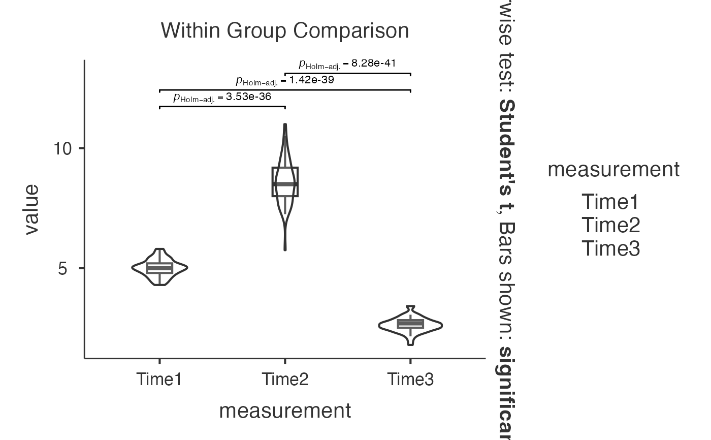
# Basic within-subjects analysis with iris dataset (simulated repeated measures)
data(iris)
iris_wide <- data.frame(
Subject = 1:50,
Time1 = iris$Sepal.Length[1:50],
Time2 = iris$Sepal.Width[1:50] * 2.5,
Time3 = iris$Petal.Length[1:50] * 1.8
)
jjwithinstats(
data = iris_wide,
dep1 = "Time1",
dep2 = "Time2",
dep3 = "Time3",
typestatistics = "parametric"
)
#>
#> VIOLIN PLOTS TO COMPARE WITHIN GROUPS
#>
#> ✅ Ready for analysis: Violin Plot comparing 3 repeated measurements.
#>
#> <div style='background-color:#f8f9fa;padding:15px;margin:10px
#> 0;border-left:4px solid #007bff;'><h4
#> style='margin-top:0;color:#007bff;'>Clinical Context
#>
#> This analysis compares 3 measurements from the same subjects. Useful
#> for: biomarker tracking, treatment response monitoring, disease
#> progression assessment.
#>
#> Test Used: Repeated measures ANOVA tests whether means differ
#> significantly across time points, assuming normal distribution.
#>
#> 🔍 What to look for:
#> • Statistical significance (p < 0.05) indicates real changes over time
#> • Effect sizes show practical importance
#> • Individual trajectories reveal response patterns
#> • Outliers may indicate treatment non-responders or measurement errors
#>
#> <div style='background-color:#f0f8f0;padding:10px;border:1px solid
#> #28a745;'>Analysis: Repeated measures ANOVA with 3 measurements per
#> subject
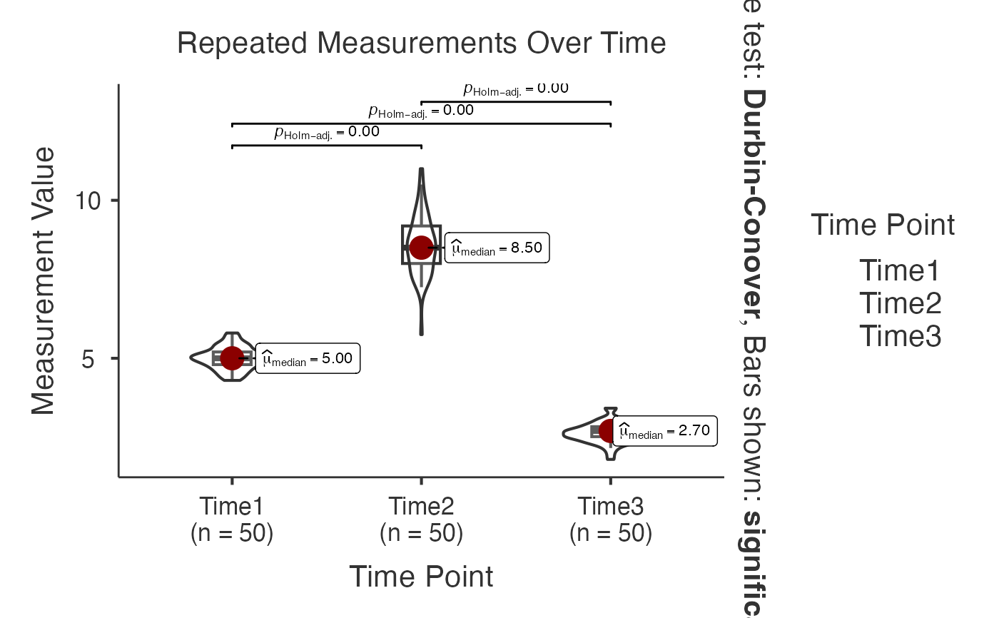
 # Advanced within-subjects analysis with custom settings
jjwithinstats(
data = iris_wide,
dep1 = "Time1",
dep2 = "Time2",
dep3 = "Time3",
typestatistics = "nonparametric",
pairwisecomparisons = TRUE,
pairwisedisplay = "significant",
centralityplotting = TRUE,
centralitytype = "nonparametric",
pointpath = TRUE,
mytitle = "Repeated Measurements Over Time",
xtitle = "Time Point",
ytitle = "Measurement Value"
)
#>
#> VIOLIN PLOTS TO COMPARE WITHIN GROUPS
#>
#> ✅ Ready for analysis: Violin Plot comparing 3 repeated measurements.
#>
#> <div style='background-color:#f8f9fa;padding:15px;margin:10px
#> 0;border-left:4px solid #007bff;'><h4
#> style='margin-top:0;color:#007bff;'>Clinical Context
#>
#> This analysis compares 3 measurements from the same subjects. Useful
#> for: biomarker tracking, treatment response monitoring, disease
#> progression assessment.
#>
#> Test Used: Friedman test compares medians across time points without
#> assuming normal distribution (robust for skewed biomarker data).
#>
#> 🔍 What to look for:
#> • Statistical significance (p < 0.05) indicates real changes over time
#> • Effect sizes show practical importance
#> • Individual trajectories reveal response patterns
#> • Outliers may indicate treatment non-responders or measurement errors
#>
#> <div style='background-color:#f0f8f0;padding:10px;border:1px solid
#> #28a745;'>Analysis: Friedman test with 3 measurements per subject
#> Configuration:
#> ✓ Pairwise comparisons enabled
#> ✓ Central tendency displayed
#> ✓ Individual trajectories shown
# Advanced within-subjects analysis with custom settings
jjwithinstats(
data = iris_wide,
dep1 = "Time1",
dep2 = "Time2",
dep3 = "Time3",
typestatistics = "nonparametric",
pairwisecomparisons = TRUE,
pairwisedisplay = "significant",
centralityplotting = TRUE,
centralitytype = "nonparametric",
pointpath = TRUE,
mytitle = "Repeated Measurements Over Time",
xtitle = "Time Point",
ytitle = "Measurement Value"
)
#>
#> VIOLIN PLOTS TO COMPARE WITHIN GROUPS
#>
#> ✅ Ready for analysis: Violin Plot comparing 3 repeated measurements.
#>
#> <div style='background-color:#f8f9fa;padding:15px;margin:10px
#> 0;border-left:4px solid #007bff;'><h4
#> style='margin-top:0;color:#007bff;'>Clinical Context
#>
#> This analysis compares 3 measurements from the same subjects. Useful
#> for: biomarker tracking, treatment response monitoring, disease
#> progression assessment.
#>
#> Test Used: Friedman test compares medians across time points without
#> assuming normal distribution (robust for skewed biomarker data).
#>
#> 🔍 What to look for:
#> • Statistical significance (p < 0.05) indicates real changes over time
#> • Effect sizes show practical importance
#> • Individual trajectories reveal response patterns
#> • Outliers may indicate treatment non-responders or measurement errors
#>
#> <div style='background-color:#f0f8f0;padding:10px;border:1px solid
#> #28a745;'>Analysis: Friedman test with 3 measurements per subject
#> Configuration:
#> ✓ Pairwise comparisons enabled
#> ✓ Central tendency displayed
#> ✓ Individual trajectories shown
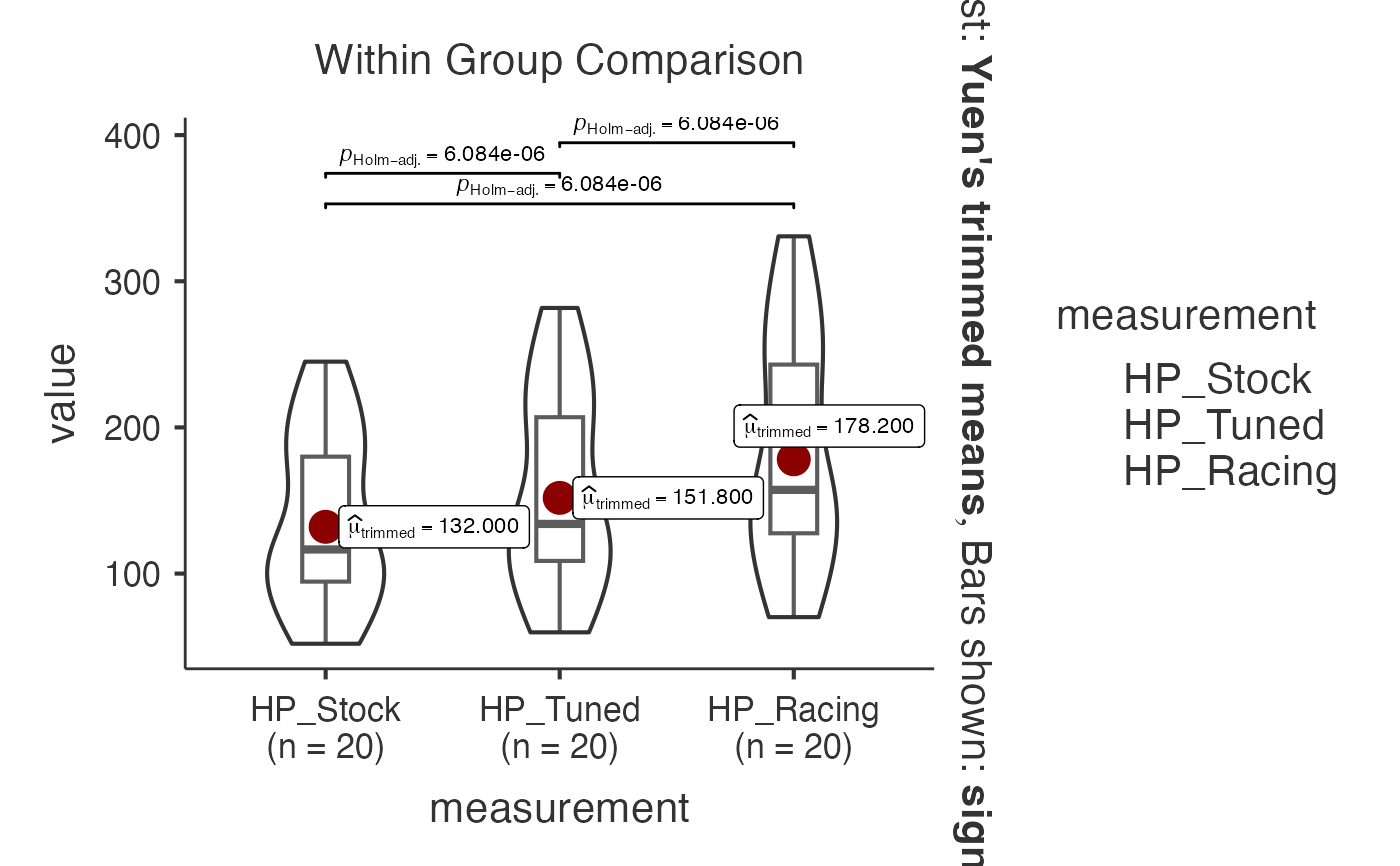
 # Robust analysis with mtcars dataset (horsepower measurements)
data(mtcars)
mtcars_wide <- data.frame(
Car = rownames(mtcars)[1:20],
HP_Stock = mtcars$hp[1:20],
HP_Tuned = mtcars$hp[1:20] * 1.15,
HP_Racing = mtcars$hp[1:20] * 1.35
)
jjwithinstats(
data = mtcars_wide,
dep1 = "HP_Stock",
dep2 = "HP_Tuned",
dep3 = "HP_Racing",
typestatistics = "robust",
centralityplotting = TRUE,
centralitytype = "robust",
effsizetype = "unbiased",
conflevel = 0.99,
k = 3
)
#>
#> VIOLIN PLOTS TO COMPARE WITHIN GROUPS
#>
#> ✅ Ready for analysis: Violin Plot comparing 3 repeated measurements.
#>
#> <div style='background-color:#f8f9fa;padding:15px;margin:10px
#> 0;border-left:4px solid #007bff;'><h4
#> style='margin-top:0;color:#007bff;'>Clinical Context
#>
#> This analysis compares 3 measurements from the same subjects. Useful
#> for: biomarker tracking, treatment response monitoring, disease
#> progression assessment.
#>
#> Test Used: Robust test uses trimmed means, reducing influence of
#> outliers common in clinical measurements.
#>
#> 🔍 What to look for:
#> • Statistical significance (p < 0.05) indicates real changes over time
#> • Effect sizes show practical importance
#> • Individual trajectories reveal response patterns
#> • Outliers may indicate treatment non-responders or measurement errors
#>
#> <div style='background-color:#f0f8f0;padding:10px;border:1px solid
#> #28a745;'>Analysis: Robust repeated measures test with 3 measurements
#> per subject
#> Configuration:
#> ✓ Central tendency displayed
# Robust analysis with mtcars dataset (horsepower measurements)
data(mtcars)
mtcars_wide <- data.frame(
Car = rownames(mtcars)[1:20],
HP_Stock = mtcars$hp[1:20],
HP_Tuned = mtcars$hp[1:20] * 1.15,
HP_Racing = mtcars$hp[1:20] * 1.35
)
jjwithinstats(
data = mtcars_wide,
dep1 = "HP_Stock",
dep2 = "HP_Tuned",
dep3 = "HP_Racing",
typestatistics = "robust",
centralityplotting = TRUE,
centralitytype = "robust",
effsizetype = "unbiased",
conflevel = 0.99,
k = 3
)
#>
#> VIOLIN PLOTS TO COMPARE WITHIN GROUPS
#>
#> ✅ Ready for analysis: Violin Plot comparing 3 repeated measurements.
#>
#> <div style='background-color:#f8f9fa;padding:15px;margin:10px
#> 0;border-left:4px solid #007bff;'><h4
#> style='margin-top:0;color:#007bff;'>Clinical Context
#>
#> This analysis compares 3 measurements from the same subjects. Useful
#> for: biomarker tracking, treatment response monitoring, disease
#> progression assessment.
#>
#> Test Used: Robust test uses trimmed means, reducing influence of
#> outliers common in clinical measurements.
#>
#> 🔍 What to look for:
#> • Statistical significance (p < 0.05) indicates real changes over time
#> • Effect sizes show practical importance
#> • Individual trajectories reveal response patterns
#> • Outliers may indicate treatment non-responders or measurement errors
#>
#> <div style='background-color:#f0f8f0;padding:10px;border:1px solid
#> #28a745;'>Analysis: Robust repeated measures test with 3 measurements
#> per subject
#> Configuration:
#> ✓ Central tendency displayed
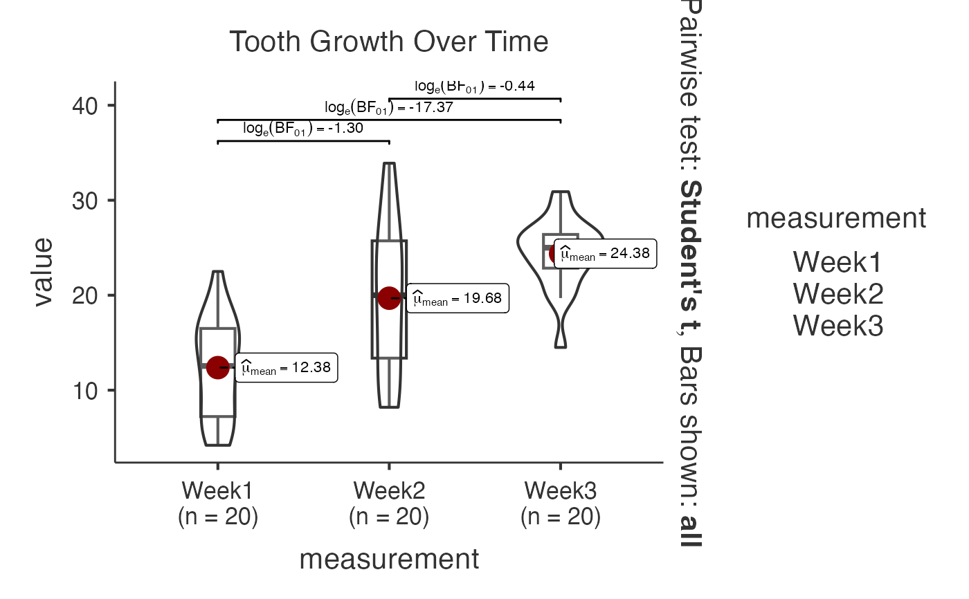
 # Bayesian analysis with ToothGrowth dataset (growth measurements)
data(ToothGrowth)
tooth_wide <- data.frame(
Subject = 1:20,
Week1 = ToothGrowth$len[1:20],
Week2 = ToothGrowth$len[21:40],
Week3 = ToothGrowth$len[41:60]
)
jjwithinstats(
data = tooth_wide,
dep1 = "Week1",
dep2 = "Week2",
dep3 = "Week3",
typestatistics = "bayes",
bfmessage = TRUE,
centralityplotting = TRUE,
mytitle = "Tooth Growth Over Time"
)
#>
#> VIOLIN PLOTS TO COMPARE WITHIN GROUPS
#>
#> ✅ Ready for analysis: Violin Plot comparing 3 repeated measurements.
#>
#> <div style='background-color:#f8f9fa;padding:15px;margin:10px
#> 0;border-left:4px solid #007bff;'><h4
#> style='margin-top:0;color:#007bff;'>Clinical Context
#>
#> This analysis compares 3 measurements from the same subjects. Useful
#> for: biomarker tracking, treatment response monitoring, disease
#> progression assessment.
#>
#> Test Used: Bayesian analysis provides evidence for/against
#> differences, useful when traditional p-values are inconclusive.
#>
#> 🔍 What to look for:
#> • Statistical significance (p < 0.05) indicates real changes over time
#> • Effect sizes show practical importance
#> • Individual trajectories reveal response patterns
#> • Outliers may indicate treatment non-responders or measurement errors
#>
#> <div style='background-color:#f0f8f0;padding:10px;border:1px solid
#> #28a745;'>Analysis: Bayesian repeated measures analysis with 3
#> measurements per subject
#> Configuration:
#> ✓ Central tendency displayed
# Bayesian analysis with ToothGrowth dataset (growth measurements)
data(ToothGrowth)
tooth_wide <- data.frame(
Subject = 1:20,
Week1 = ToothGrowth$len[1:20],
Week2 = ToothGrowth$len[21:40],
Week3 = ToothGrowth$len[41:60]
)
jjwithinstats(
data = tooth_wide,
dep1 = "Week1",
dep2 = "Week2",
dep3 = "Week3",
typestatistics = "bayes",
bfmessage = TRUE,
centralityplotting = TRUE,
mytitle = "Tooth Growth Over Time"
)
#>
#> VIOLIN PLOTS TO COMPARE WITHIN GROUPS
#>
#> ✅ Ready for analysis: Violin Plot comparing 3 repeated measurements.
#>
#> <div style='background-color:#f8f9fa;padding:15px;margin:10px
#> 0;border-left:4px solid #007bff;'><h4
#> style='margin-top:0;color:#007bff;'>Clinical Context
#>
#> This analysis compares 3 measurements from the same subjects. Useful
#> for: biomarker tracking, treatment response monitoring, disease
#> progression assessment.
#>
#> Test Used: Bayesian analysis provides evidence for/against
#> differences, useful when traditional p-values are inconclusive.
#>
#> 🔍 What to look for:
#> • Statistical significance (p < 0.05) indicates real changes over time
#> • Effect sizes show practical importance
#> • Individual trajectories reveal response patterns
#> • Outliers may indicate treatment non-responders or measurement errors
#>
#> <div style='background-color:#f0f8f0;padding:10px;border:1px solid
#> #28a745;'>Analysis: Bayesian repeated measures analysis with 3
#> measurements per subject
#> Configuration:
#> ✓ Central tendency displayed