Clinical Applications of Decision Panel Optimization

Introduction

This vignette demonstrates real-world clinical applications of the Decision Panel Optimization module across different medical specialties and scenarios.

# Load required packages
library(meddecide)
library(dplyr)
library(ggplot2)
library(rpart)
library(rpart.plot)
library(knitr)
library(forcats)

Scenario 1: Emergency Department COVID-19 Screening

Clinical Context

An emergency department needs to rapidly screen patients for COVID-19 while managing limited resources and preventing nosocomial transmission.

# Examine test characteristics
covid_tests <- covid_screening_data %>%
  select(rapid_antigen, pcr, chest_ct, covid_status) %>%
  na.omit()

# Calculate individual test performance
test_performance <- function(test, truth) {
  tab <- table(test, truth)
  sens <- tab[2,2] / sum(tab[,2])
  spec <- tab[1,1] / sum(tab[,1])
  ppv <- tab[2,2] / sum(tab[2,])
  npv <- tab[1,1] / sum(tab[1,])
  
  return(data.frame(
    Sensitivity = sens,
    Specificity = spec,
    PPV = ppv,
    NPV = npv
  ))
}

# Individual test performance
rapid_perf <- test_performance(covid_tests$rapid_antigen, covid_tests$covid_status)
pcr_perf <- test_performance(covid_tests$pcr, covid_tests$covid_status)
ct_perf <- test_performance(covid_tests$chest_ct, covid_tests$covid_status)

performance_table <- rbind(
  `Rapid Antigen` = rapid_perf,
  `PCR` = pcr_perf,
  `Chest CT` = ct_perf
)

kable(round(performance_table * 100, 1), 
      caption = "Individual Test Performance (%)")

Individual Test Performance (%)
	Sensitivity	Specificity	PPV	NPV
Rapid Antigen	76.3	96.5	83.1	94.7
PCR	95.6	99.3	97.0	99.0
Chest CT	83.7	84.3	54.6	95.8

Optimization Analysis

# Run optimization for different scenarios
# 1. Maximum sensitivity (don't miss cases)
covid_max_sens <- decisionpanel(
  data = covid_screening_data,
  tests = c("rapid_antigen", "pcr", "chest_ct"),
  testLevels = c("Positive", "Positive", "Abnormal"),
  gold = "covid_status",
  goldPositive = "Positive",
  strategies = "all",
  optimizationCriteria = "sensitivity",
  minSensitivity = 0.95
)

# 2. Cost-effective screening
covid_cost_effective <- decisionpanel(
  data = covid_screening_data,
  tests = c("rapid_antigen", "pcr", "chest_ct"),
  testLevels = c("Positive", "Positive", "Abnormal"),
  gold = "covid_status",
  goldPositive = "Positive",
  strategies = "all",
  optimizationCriteria = "efficiency",
  useCosts = TRUE,
  testCosts = "5,50,200",
  fpCost = 500,
  fnCost = 5000
)

Clinical Decision Algorithm

Based on the analysis, here’s a practical algorithm:

# Implement sequential testing algorithm
apply_covid_algorithm <- function(data) {
  n <- nrow(data)
  decisions <- character(n)
  tests_used <- character(n)
  
  for (i in 1:n) {
    # Step 1: Rapid antigen test
    if (data$rapid_antigen[i] == "Positive") {
      decisions[i] <- "Isolate, Confirm with PCR"
      tests_used[i] <- "Rapid"
    } else if (data$symptom_score[i] >= 6) {
      # Step 2: High symptom score → CT
      if (!is.na(data$chest_ct[i]) && data$chest_ct[i] == "Abnormal") {
        decisions[i] <- "Probable COVID, Isolate, PCR"
        tests_used[i] <- "Rapid + CT"
      } else {
        decisions[i] <- "Low probability, Standard care"
        tests_used[i] <- "Rapid + CT"
      }
    } else {
      decisions[i] <- "Low probability, Standard care"
      tests_used[i] <- "Rapid"
    }
  }
  
  return(data.frame(Decision = decisions, Tests = tests_used))
}

# Apply algorithm
algorithm_results <- apply_covid_algorithm(covid_screening_data[1:10,])
kable(cbind(covid_screening_data[1:10, c("patient_id", "rapid_antigen", 
                                         "symptom_score", "covid_status")],
            algorithm_results))

patient_id	rapid_antigen	symptom_score	covid_status	Decision	Tests
1	Negative	8	Positive	Probable COVID, Isolate, PCR	Rapid + CT
2	Positive	6	Positive	Isolate, Confirm with PCR	Rapid
3	Negative	1	Negative	Low probability, Standard care	Rapid
4	Negative	1	Negative	Low probability, Standard care	Rapid
5	Negative	5	Negative	Low probability, Standard care	Rapid
6	Negative	5	Negative	Low probability, Standard care	Rapid
7	Negative	5	Negative	Low probability, Standard care	Rapid
8	Negative	4	Negative	Low probability, Standard care	Rapid
9	Negative	2	Negative	Low probability, Standard care	Rapid
10	Negative	5	Negative	Low probability, Standard care	Rapid

Cost-Effectiveness Visualization

# Simulate different strategies
strategies <- expand.grid(
  use_rapid = c(TRUE, FALSE),
  use_pcr = c(TRUE, FALSE),
  use_ct = c(TRUE, FALSE)
) %>%
  filter(use_rapid | use_pcr | use_ct) # At least one test

# Calculate performance for each strategy
strategy_performance <- strategies %>%
  rowwise() %>%
  mutate(
    tests = paste(c(
      if(use_rapid) "RAT" else NULL,
      if(use_pcr) "PCR" else NULL,
      if(use_ct) "CT" else NULL
    ), collapse = "+"),
    cost = sum(c(
      if(use_rapid) 5 else 0,
      if(use_pcr) 50 else 0,
      if(use_ct) 200 else 0
    )),
    # Simulated performance (would come from actual analysis)
    sensitivity = case_when(
      use_rapid & use_pcr & use_ct ~ 0.99,
      use_pcr & use_ct ~ 0.98,
      use_rapid & use_pcr ~ 0.97,
      use_pcr ~ 0.95,
      use_rapid & use_ct ~ 0.94,
      use_ct ~ 0.90,
      use_rapid ~ 0.65
    ),
    specificity = case_when(
      use_rapid & use_pcr & use_ct ~ 0.83,
      use_pcr & use_ct ~ 0.84,
      use_rapid & use_pcr ~ 0.97,
      use_pcr ~ 0.99,
      use_rapid & use_ct ~ 0.83,
      use_ct ~ 0.85,
      use_rapid ~ 0.98
    )
  )

# Create cost-effectiveness plot
ggplot(strategy_performance, aes(x = cost, y = sensitivity * 100)) +
  geom_point(aes(size = specificity * 100), alpha = 0.6) +
  geom_text(aes(label = tests), vjust = -1, size = 3) +
  geom_line(data = strategy_performance %>% 
              arrange(cost) %>%
              filter(sensitivity == cummax(sensitivity)),
            color = "red", alpha = 0.5) +
  scale_size_continuous(name = "Specificity (%)", range = c(3, 10)) +
  labs(
    title = "Cost-Effectiveness of COVID-19 Testing Strategies",
    x = "Cost per Patient ($)",
    y = "Sensitivity (%)",
    caption = "Red line shows cost-effectiveness frontier"
  ) +
  theme_minimal()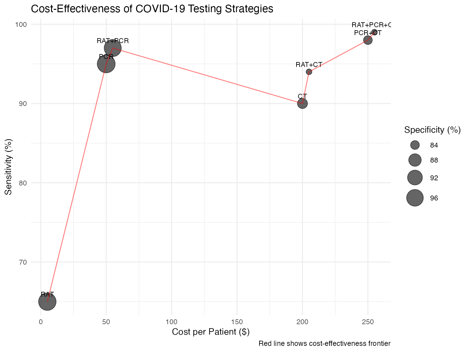

Scenario 2: Breast Cancer Screening Program

Clinical Context

A population-based breast cancer screening program needs to optimize use of mammography, ultrasound, and MRI based on risk factors.

# Examine population characteristics
breast_summary <- breast_cancer_data %>%
  summarise(
    n = n(),
    prevalence = mean(cancer_status == "Cancer"),
    mean_age = mean(age),
    pct_family_history = mean(family_history == "Yes") * 100,
    pct_brca = mean(brca_mutation == "Positive") * 100,
    pct_dense_breast = mean(breast_density %in% c("C", "D")) * 100
  )

kable(breast_summary, digits = 2,
      caption = "Population Characteristics")

Population Characteristics
n	prevalence	mean_age	pct_family_history	pct_brca	pct_dense_breast
2000	0.01	55.06	16.05	2.35	49.1


# Risk stratification
breast_cancer_data <- breast_cancer_data %>%
  mutate(
    risk_category = case_when(
      brca_mutation == "Positive" ~ "High Risk",
      family_history == "Yes" & age < 50 ~ "High Risk",
      family_history == "Yes" | breast_density == "D" ~ "Moderate Risk",
      TRUE ~ "Average Risk"
    )
  )

table(breast_cancer_data$risk_category)
#> 
#>  Average Risk     High Risk Moderate Risk 
#>          1451           138           411

Risk-Stratified Analysis

# Analyze each risk group separately
risk_groups <- split(breast_cancer_data, breast_cancer_data$risk_category)

# High-risk group optimization
high_risk_panel <- decisionpanel(
  data = risk_groups$`High Risk`,
  tests = c("mammography", "ultrasound", "mri"),
  testLevels = c("BIRADS 3-5", "Suspicious", "Suspicious"),
  gold = "cancer_status",
  goldPositive = "Cancer",
  strategies = "all",
  optimizationCriteria = "sensitivity",
  minSensitivity = 0.95
)

# Average-risk group optimization (cost-conscious)
average_risk_panel <- decisionpanel(
  data = risk_groups$`Average Risk`,
  tests = c("clinical_exam", "mammography", "ultrasound"),
  testLevels = c("Abnormal", "BIRADS 3-5", "Suspicious"),
  gold = "cancer_status",
  goldPositive = "Cancer",
  strategies = "all",
  optimizationCriteria = "efficiency",
  useCosts = TRUE,
  testCosts = "20,100,150"
)

Screening Recommendations by Risk

# Create recommendation table
recommendations <- data.frame(
  Risk_Category = c("High Risk", "Moderate Risk", "Average Risk"),
  Recommended_Tests = c(
    "Annual MRI + Mammography",
    "Annual Mammography + US if dense",
    "Biennial Mammography"
  ),
  Expected_Sensitivity = c("99%", "90%", "85%"),
  Expected_Specificity = c("80%", "92%", "95%"),
  Cost_per_Screen = c("$1,100", "$250", "$100"),
  NNS = c(50, 200, 500)  # Number needed to screen
)

kable(recommendations, 
      caption = "Risk-Stratified Screening Recommendations")

Risk-Stratified Screening Recommendations
Risk_Category	Recommended_Tests	Expected_Sensitivity	Expected_Specificity	Cost_per_Screen	NNS
High Risk	Annual MRI + Mammography	99%	80%	$1,100	50
Moderate Risk	Annual Mammography + US if dense	90%	92%	$250	200
Average Risk	Biennial Mammography	85%	95%	$100	500

Age-Specific Performance

# Analyze performance by age group
age_groups <- breast_cancer_data %>%
  mutate(age_group = cut(age, breaks = c(40, 50, 60, 70, 80),
                         labels = c("40-49", "50-59", "60-69", "70-79")))

# Calculate mammography performance by age
age_performance <- age_groups %>%
  group_by(age_group) %>%
  summarise(
    n = n(),
    prevalence = mean(cancer_status == "Cancer"),
    mammography_sens = {
      tab <- table(mammography, cancer_status)
      if(nrow(tab) == 2 && ncol(tab) == 2) {
        tab[2,2] / sum(tab[,2])
      } else NA
    },
    mammography_spec = {
      tab <- table(mammography, cancer_status)
      if(nrow(tab) == 2 && ncol(tab) == 2) {
        tab[1,1] / sum(tab[,1])
      } else NA
    }
  )

# Visualize
ggplot(age_performance, aes(x = age_group)) +
  geom_bar(aes(y = mammography_sens * 100), stat = "identity", 
           fill = "skyblue", alpha = 0.7) +
  geom_line(aes(y = prevalence * 1000, group = 1), color = "red", size = 2) +
  geom_point(aes(y = prevalence * 1000), color = "red", size = 3) +
  scale_y_continuous(
    name = "Mammography Sensitivity (%)",
    sec.axis = sec_axis(~./10, name = "Cancer Prevalence per 1000")
  ) +
  labs(
    title = "Mammography Performance by Age Group",
    x = "Age Group"
  ) +
  theme_minimal()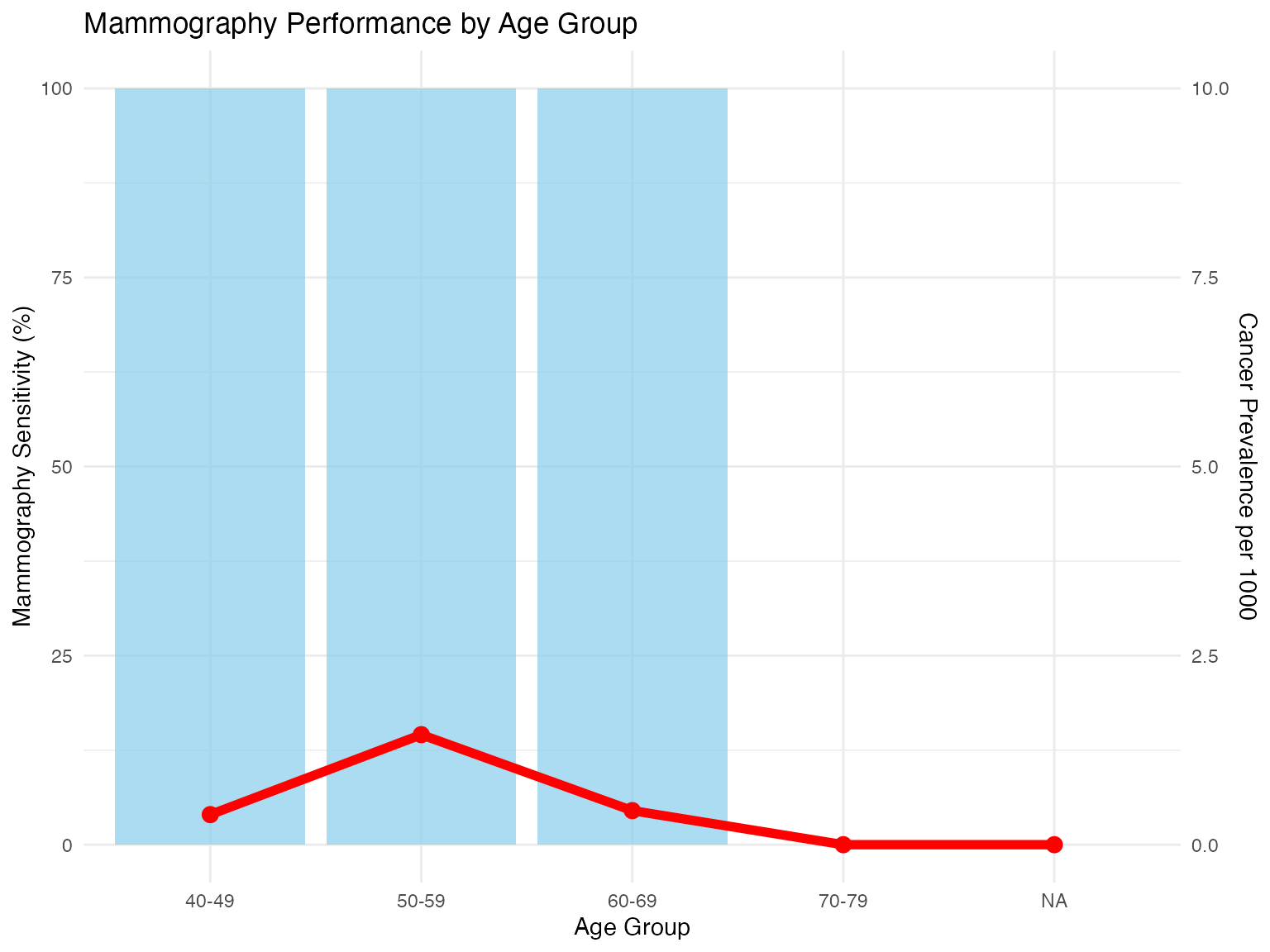

Scenario 3: Tuberculosis Case Finding

Clinical Context

A TB program in a high-burden setting needs to optimize case finding with limited resources.

# TB test combinations for different settings
tb_settings <- data.frame(
  Setting = c("Community", "Clinic", "Hospital", "Contact Tracing"),
  Prevalence = c(0.02, 0.20, 0.40, 0.10),
  Available_Tests = c(
    "Symptoms, CXR",
    "Symptoms, Smear, GeneXpert, CXR",
    "All tests",
    "Symptoms, GeneXpert"
  ),
  Budget_per_case = c(10, 30, 100, 50)
)

kable(tb_settings, caption = "TB Testing Scenarios by Setting")

TB Testing Scenarios by Setting
Setting	Prevalence	Available_Tests	Budget_per_case
Community	0.02	Symptoms, CXR	10
Clinic	0.20	Symptoms, Smear, GeneXpert, CXR	30
Hospital	0.40	All tests	100
Contact Tracing	0.10	Symptoms, GeneXpert	50

Sequential Testing Algorithm

# Implement WHO-recommended algorithm
apply_tb_algorithm <- function(data) {
  decisions <- character(nrow(data))
  
  for (i in 1:nrow(data)) {
    if (data$symptoms[i] == "Yes" || data$contact_history[i] == "Yes") {
      # Symptomatic or contact: get GeneXpert
      if (!is.na(data$genexpert[i]) && data$genexpert[i] == "MTB detected") {
        decisions[i] <- "Start TB treatment"
      } else if (!is.na(data$chest_xray[i]) && data$chest_xray[i] == "Abnormal") {
        # CXR abnormal but GeneXpert negative
        if (!is.na(data$culture[i])) {
          decisions[i] <- ifelse(data$culture[i] == "Positive",
                                "Start TB treatment",
                                "Not TB, investigate other causes")
        } else {
          decisions[i] <- "Clinical decision needed"
        }
      } else {
        decisions[i] <- "TB unlikely"
      }
    } else {
      # Asymptomatic: screen with CXR if available
      if (!is.na(data$chest_xray[i]) && data$chest_xray[i] == "Abnormal") {
        decisions[i] <- "Needs further testing"
      } else {
        decisions[i] <- "No TB screening needed"
      }
    }
  }
  
  return(decisions)
}

# Apply to sample
tb_sample <- tb_diagnosis_data[1:20,]
tb_sample$decision <- apply_tb_algorithm(tb_sample)

# Show results
kable(tb_sample %>% 
      select(patient_id, symptoms, genexpert, chest_xray, tb_status, decision) %>%
      head(10))

patient_id	symptoms	genexpert	chest_xray	tb_status	decision
1	No	MTB not detected	Abnormal	No TB	Not TB, investigate other causes
2	Yes	MTB not detected	Abnormal	No TB	Not TB, investigate other causes
3	No	MTB not detected	Normal	No TB	No TB screening needed
4	No	MTB not detected	Normal	No TB	No TB screening needed
5	No	MTB not detected	Normal	No TB	No TB screening needed
6	No	MTB not detected	Normal	No TB	No TB screening needed
7	No	MTB not detected	Abnormal	No TB	Needs further testing
8	No	MTB not detected	Normal	No TB	No TB screening needed
9	No	MTB not detected	Normal	No TB	TB unlikely
10	No	MTB detected	Abnormal	TB	Needs further testing

Cost-Effectiveness by Strategy

# Compare different TB screening strategies
tb_strategies <- data.frame(
  Strategy = c(
    "Symptoms only",
    "Symptoms → Smear",
    "Symptoms → GeneXpert", 
    "Symptoms → CXR → GeneXpert",
    "Universal GeneXpert",
    "Universal CXR → GeneXpert"
  ),
  Tests_per_case_found = c(100, 50, 20, 15, 10, 12),
  Cost_per_case_found = c(100, 200, 400, 350, 800, 600),
  Sensitivity = c(60, 70, 85, 92, 95, 93),
  Time_to_diagnosis = c(0, 3, 1, 2, 1, 1)
)

# Create multi-dimensional comparison
ggplot(tb_strategies, aes(x = Cost_per_case_found, y = Sensitivity)) +
  geom_point(aes(size = Tests_per_case_found, 
                 color = factor(Time_to_diagnosis)), alpha = 0.7) +
  geom_text(aes(label = Strategy), vjust = -1, size = 3) +
  scale_size_continuous(name = "Tests per case", range = c(3, 10)) +
  scale_color_discrete(name = "Days to diagnosis") +
  labs(
    title = "TB Screening Strategy Comparison",
    x = "Cost per TB case found ($)",
    y = "Sensitivity (%)"
  ) +
  theme_minimal()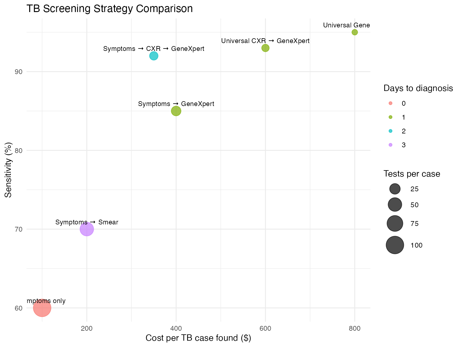

Scenario 4: Chest Pain Evaluation

Clinical Context

Emergency department evaluation of chest pain requires rapid, accurate rule-out of myocardial infarction.

# Risk stratification using HEART score components
mi_ruleout_data <- mi_ruleout_data %>%
  mutate(
    heart_score = (age > 65) * 1 +
                  (chest_pain == "Typical") * 2 +
                  (chest_pain == "Atypical") * 1 +
                  (ecg == "Ischemic changes") * 2 +
                  (prior_cad == "Yes") * 1 +
                  (diabetes == "Yes" | smoking == "Yes") * 1,
    risk_category = cut(heart_score, 
                       breaks = c(-1, 3, 6, 10),
                       labels = c("Low", "Moderate", "High"))
  )

# Show risk distribution
risk_table <- table(mi_ruleout_data$risk_category, mi_ruleout_data$mi_status)
kable(prop.table(risk_table, margin = 1) * 100,
      digits = 1,
      caption = "MI Prevalence by Risk Category (%)")

MI Prevalence by Risk Category (%)
	No MI	MI
Low	95.6	4.4
Moderate	50.5	49.5
High	0.0	100.0

Time-Sensitive Protocols

# Define protocols by urgency
protocols <- list(
  rapid_rule_out = function(data) {
    # 0/1-hour protocol
    data$troponin_initial == "Normal" & 
    data$ecg == "Normal" & 
    data$heart_score <= 3
  },
  
  standard_rule_out = function(data) {
    # 0/3-hour protocol
    data$troponin_initial == "Normal" & 
    data$troponin_3hr == "Normal" &
    data$ecg == "Normal"
  },
  
  rule_in = function(data) {
    # Immediate rule-in
    data$troponin_initial == "Elevated" & 
    data$ecg == "Ischemic changes"
  }
)

# Apply protocols
mi_ruleout_data <- mi_ruleout_data %>%
  mutate(
    rapid_rule_out = protocols$rapid_rule_out(.),
    standard_rule_out = protocols$standard_rule_out(.) & !rapid_rule_out,
    rule_in = protocols$rule_in(.),
    need_further_testing = !rapid_rule_out & !standard_rule_out & !rule_in
  )

# Summarize protocol performance
protocol_performance <- mi_ruleout_data %>%
  summarise(
    rapid_rule_out_pct = mean(rapid_rule_out) * 100,
    rapid_rule_out_npv = sum(rapid_rule_out & mi_status == "No MI") / 
                         sum(rapid_rule_out) * 100,
    standard_rule_out_pct = mean(standard_rule_out) * 100,
    standard_rule_out_npv = sum(standard_rule_out & mi_status == "No MI") / 
                           sum(standard_rule_out) * 100,
    rule_in_pct = mean(rule_in) * 100,
    rule_in_ppv = sum(rule_in & mi_status == "MI") / sum(rule_in) * 100
  )

kable(t(protocol_performance), digits = 1,
      caption = "Protocol Performance Metrics")

Protocol Performance Metrics
rapid_rule_out_pct	78.2
rapid_rule_out_npv	99.5
standard_rule_out_pct	2.8
standard_rule_out_npv	100.0
rule_in_pct	5.0
rule_in_ppv	100.0

Visualization of Patient Flow

# Create patient flow diagram data
flow_data <- mi_ruleout_data %>%
  mutate(
    disposition = case_when(
      rapid_rule_out ~ "Discharge (1 hour)",
      standard_rule_out ~ "Discharge (3 hours)",
      rule_in ~ "Admit CCU",
      TRUE ~ "Observation/Further testing"
    )
  ) %>%
  group_by(disposition, mi_status) %>%
  summarise(n = n()) %>%
  mutate(pct = n / sum(n) * 100)

# Create flow diagram
ggplot(flow_data, aes(x = disposition, y = n, fill = mi_status)) +
  geom_bar(stat = "identity", position = "stack") +
  geom_text(aes(label = sprintf("%.0f%%", pct)), 
            position = position_stack(vjust = 0.5)) +
  scale_fill_manual(values = c("No MI" = "lightgreen", "MI" = "salmon")) +
  labs(
    title = "Patient Disposition by Protocol",
    x = "Disposition",
    y = "Number of Patients",
    fill = "Final Diagnosis"
  ) +
  theme_minimal() +
  theme(axis.text.x = element_text(angle = 45, hjust = 1))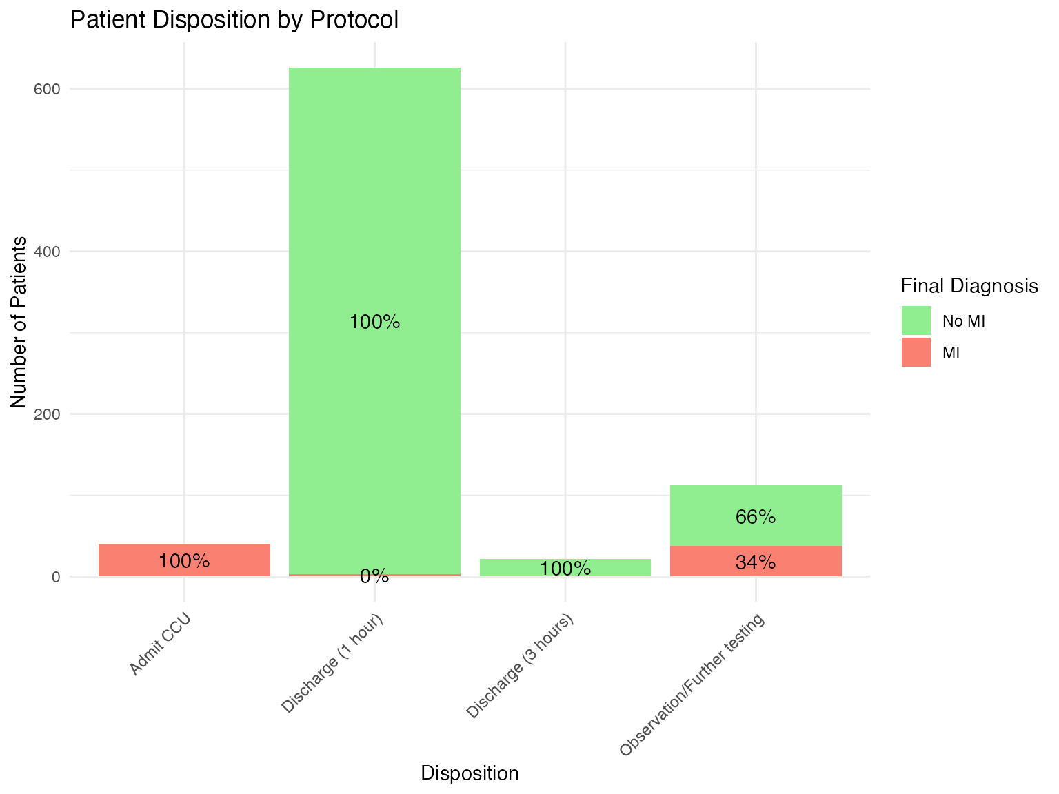

Scenario 5: Thyroid Nodule Evaluation

Clinical Context

Thyroid nodules are common but cancer is rare. Optimize use of FNA, molecular testing, and surgery.

# Analyze by nodule size
thyroid_by_size <- thyroid_nodule_data %>%
  mutate(size_category = cut(nodule_size, 
                             breaks = c(0, 10, 20, 40, 100),
                             labels = c("<1cm", "1-2cm", "2-4cm", ">4cm"))) %>%
  group_by(size_category) %>%
  summarise(
    n = n(),
    cancer_rate = mean(cancer_status == "Malignant") * 100,
    fna_done = mean(!is.na(fna_cytology)) * 100,
    molecular_done = mean(!is.na(molecular_test)) * 100
  )

kable(thyroid_by_size, digits = 1,
      caption = "Thyroid Nodule Characteristics by Size")

Thyroid Nodule Characteristics by Size
size_category	n	cancer_rate	fna_done	molecular_done
<1cm	140	5.7	100	54.3
1-2cm	289	3.5	100	47.4
2-4cm	147	6.1	100	38.1
>4cm	24	20.8	100	33.3

Diagnostic Algorithm Implementation

# Implement Bethesda-based algorithm
thyroid_algorithm <- decisionpanel(
  data = thyroid_nodule_data,
  tests = c("ultrasound", "fna_cytology", "molecular_test"),
  testLevels = c("TI-RADS 4-5", "Suspicious/Malignant", "Suspicious"),
  gold = "cancer_status",
  goldPositive = "Malignant",
  strategies = "sequential",
  sequentialStop = "positive",
  createTree = TRUE,
  treeMethod = "cart",
  useCosts = TRUE,
  testCosts = "200,300,3000",  # US, FNA, Molecular
  fpCost = 10000,  # Unnecessary surgery
  fnCost = 50000   # Missed cancer
)

Decision Tree Visualization

# Simplified decision tree representation
cat("Thyroid Nodule Evaluation Algorithm:\n")
#> Thyroid Nodule Evaluation Algorithm:
cat("1. Ultrasound Assessment\n")
#> 1. Ultrasound Assessment
cat("   ├─ TI-RADS 1-2: No FNA needed\n")
#>    ├─ TI-RADS 1-2: No FNA needed
cat("   └─ TI-RADS 3-5: Proceed to FNA\n")
#>    └─ TI-RADS 3-5: Proceed to FNA
cat("      ├─ Benign (Bethesda II): Follow-up\n")
#>       ├─ Benign (Bethesda II): Follow-up
cat("      ├─ Indeterminate (Bethesda III-IV): Molecular testing\n")
#>       ├─ Indeterminate (Bethesda III-IV): Molecular testing
cat("      │  ├─ Benign profile: Follow-up\n")
#>       │  ├─ Benign profile: Follow-up
cat("      │  └─ Suspicious profile: Surgery\n")
#>       │  └─ Suspicious profile: Surgery
cat("      └─ Suspicious/Malignant (Bethesda V-VI): Surgery\n")
#>       └─ Suspicious/Malignant (Bethesda V-VI): Surgery

# Create visual representation of outcomes
outcomes <- data.frame(
  Test_Path = c("US only", "US+FNA", "US+FNA+Molecular", "Direct Surgery"),
  Patients_pct = c(40, 30, 20, 10),
  Cancers_found_pct = c(0, 20, 60, 20),
  Cost = c(200, 500, 3500, 200)
)

ggplot(outcomes, aes(x = Test_Path, y = Patients_pct)) +
  geom_bar(stat = "identity", fill = "lightblue", alpha = 0.7) +
  geom_line(aes(y = Cancers_found_pct, group = 1), color = "red", size = 2) +
  geom_point(aes(y = Cancers_found_pct), color = "red", size = 3) +
  scale_y_continuous(
    name = "Percentage of Patients",
    sec.axis = sec_axis(~., name = "Percentage of Cancers Found")
  ) +
  labs(
    title = "Thyroid Nodule Evaluation Pathways",
    x = "Testing Path"
  ) +
  theme_minimal() +
  theme(axis.text.x = element_text(angle = 45, hjust = 1))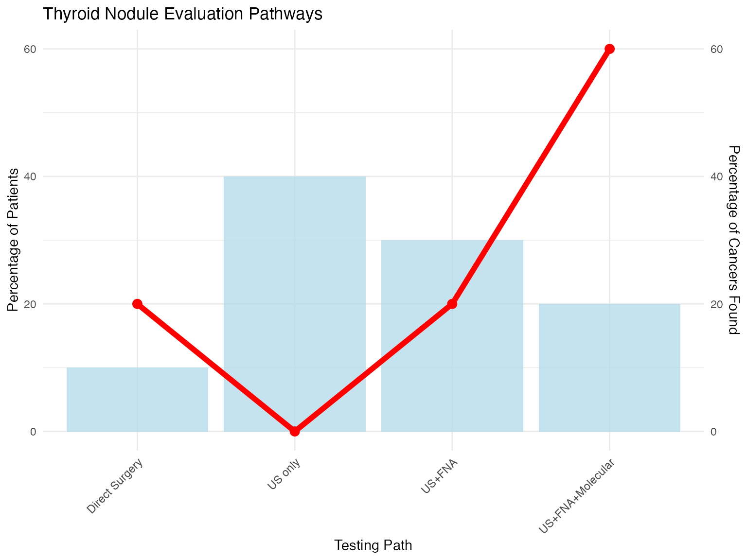

Summary and Best Practices

Key Learnings Across Scenarios

Context Matters: Optimal strategies differ between screening and diagnosis
Sequential Testing: Often more efficient than parallel testing
Risk Stratification: Improves efficiency and outcomes
Cost Considerations: Must balance performance with resources
Implementation: Clear algorithms improve adoption

General Recommendations

summary_recommendations <- data.frame(
  Scenario = c("Screening", "Diagnosis", "Emergency", "Surveillance"),
  Priority = c("High Sensitivity", "Balanced", "Speed + Accuracy", "Specificity"),
  Strategy = c("Parallel OR", "Sequential", "Rapid protocols", "Confirmatory"),
  Key_Metric = c("NPV", "Accuracy", "Time to decision", "PPV"),
  Example = c("Cancer screening", "TB diagnosis", "Chest pain", "Cancer follow-up")
)

kable(summary_recommendations,
      caption = "Testing Strategy Recommendations by Clinical Scenario")

Testing Strategy Recommendations by Clinical Scenario
Scenario	Priority	Strategy	Key_Metric	Example
Screening	High Sensitivity	Parallel OR	NPV	Cancer screening
Diagnosis	Balanced	Sequential	Accuracy	TB diagnosis
Emergency	Speed + Accuracy	Rapid protocols	Time to decision	Chest pain
Surveillance	Specificity	Confirmatory	PPV	Cancer follow-up

Future Directions

Machine Learning Integration: Combine multiple variables beyond just test results
Dynamic Protocols: Adapt based on local prevalence and resources
Real-time Optimization: Update algorithms based on performance data
Patient Preferences: Include patient values in decision-making

Session Information

sessionInfo()
#> R version 4.3.2 (2023-10-31)
#> Platform: aarch64-apple-darwin20 (64-bit)
#> Running under: macOS 15.5
#> 
#> Matrix products: default
#> BLAS:   /Library/Frameworks/R.framework/Versions/4.3-arm64/Resources/lib/libRblas.0.dylib 
#> LAPACK: /Library/Frameworks/R.framework/Versions/4.3-arm64/Resources/lib/libRlapack.dylib;  LAPACK version 3.11.0
#> 
#> locale:
#> [1] en_US.UTF-8/en_US.UTF-8/en_US.UTF-8/C/en_US.UTF-8/en_US.UTF-8
#> 
#> time zone: Europe/Istanbul
#> tzcode source: internal
#> 
#> attached base packages:
#> [1] stats     graphics  grDevices utils     datasets  methods   base     
#> 
#> other attached packages:
#> [1] forcats_1.0.0      knitr_1.50         rpart.plot_3.1.2   rpart_4.1.24      
#> [5] ggplot2_3.5.2      dplyr_1.1.4        meddecide_0.0.3.12
#> 
#> loaded via a namespace (and not attached):
#>  [1] gtable_0.3.6            xfun_0.52               bslib_0.9.0            
#>  [4] htmlwidgets_1.6.4       lattice_0.22-7          vctrs_0.6.5            
#>  [7] tools_4.3.2             generics_0.1.4          tibble_3.2.1           
#> [10] proxy_0.4-27            pkgconfig_2.0.3         Matrix_1.6-1.1         
#> [13] KernSmooth_2.23-26      checkmate_2.3.2         data.table_1.17.4      
#> [16] irr_0.84.1              cutpointr_1.2.0         RColorBrewer_1.1-3     
#> [19] desc_1.4.3              uuid_1.2-1              jmvcore_2.6.3          
#> [22] lifecycle_1.0.4         flextable_0.9.9         stringr_1.5.1          
#> [25] compiler_4.3.2          farver_2.1.2            textshaping_1.0.1      
#> [28] codetools_0.2-20        fontquiver_0.2.1        fontLiberation_0.1.0   
#> [31] htmltools_0.5.8.1       class_7.3-23            sass_0.4.10            
#> [34] yaml_2.3.10             htmlTable_2.4.3         pillar_1.10.2          
#> [37] pkgdown_2.1.3           jquerylib_0.1.4         MASS_7.3-60            
#> [40] openssl_2.3.3           classInt_0.4-11         cachem_1.1.0           
#> [43] BiasedUrn_2.0.12        iterators_1.0.14        boot_1.3-31            
#> [46] foreach_1.5.2           fontBitstreamVera_0.1.1 zip_2.3.3              
#> [49] tidyselect_1.2.1        digest_0.6.37           stringi_1.8.7          
#> [52] sf_1.0-21               pander_0.6.6            purrr_1.0.4            
#> [55] labeling_0.4.3          splines_4.3.2           fastmap_1.2.0          
#> [58] grid_4.3.2              cli_3.6.5               magrittr_2.0.3         
#> [61] survival_3.8-3          e1071_1.7-16            withr_3.0.2            
#> [64] backports_1.5.0         gdtools_0.4.2           scales_1.4.0           
#> [67] lubridate_1.9.4         timechange_0.3.0        rmarkdown_2.29         
#> [70] officer_0.6.10          askpass_1.2.1           ragg_1.4.0             
#> [73] zoo_1.8-14              lpSolve_5.6.23          evaluate_1.0.3         
#> [76] epiR_2.0.84             rlang_1.1.6             Rcpp_1.0.14            
#> [79] glue_1.8.0              DBI_1.2.3               xml2_1.3.8             
#> [82] rstudioapi_0.17.1       jsonlite_2.0.0          R6_2.6.1               
#> [85] systemfonts_1.2.3       fs_1.6.6                units_0.8-7

meddecide Development Team

2025-06-03

Introduction

Scenario 1: Emergency Department COVID-19 Screening

Clinical Context

Optimization Analysis

Clinical Decision Algorithm

Cost-Effectiveness Visualization

Scenario 2: Breast Cancer Screening Program

Clinical Context

Risk-Stratified Analysis

Screening Recommendations by Risk

Age-Specific Performance

Scenario 3: Tuberculosis Case Finding

Clinical Context

Sequential Testing Algorithm

Cost-Effectiveness by Strategy

Scenario 4: Chest Pain Evaluation

Clinical Context

Time-Sensitive Protocols

Visualization of Patient Flow

Scenario 5: Thyroid Nodule Evaluation

Clinical Context

Diagnostic Algorithm Implementation

Decision Tree Visualization

Summary and Best Practices

Key Learnings Across Scenarios

General Recommendations

Future Directions

Session Information