Advanced Features and Customization in Decision Panel Optimization

Introduction

This vignette covers advanced features of the Decision Panel Optimization module, including custom optimization functions, complex constraints, and programmatic access to results.

# Load required packages
library(ClinicoPath)
#> Registered S3 method overwritten by 'future':
#>   method               from      
#>   all.equal.connection parallelly
#> Warning: replacing previous import 'dplyr::select' by 'jmvcore::select' when
#> loading 'ClinicoPath'
#> Warning: replacing previous import 'cutpointr::roc' by 'pROC::roc' when loading
#> 'ClinicoPath'
#> Warning: replacing previous import 'cutpointr::auc' by 'pROC::auc' when loading
#> 'ClinicoPath'
#> Warning: replacing previous import 'magrittr::extract' by 'tidyr::extract' when
#> loading 'ClinicoPath'
#> Warning in check_dep_version(): ABI version mismatch: 
#> lme4 was built with Matrix ABI version 1
#> Current Matrix ABI version is 0
#> Please re-install lme4 from source or restore original 'Matrix' package
#> Warning: replacing previous import 'jmvcore::select' by 'dplyr::select' when
#> loading 'ClinicoPath'
#> Registered S3 methods overwritten by 'ggpp':
#>   method                  from   
#>   heightDetails.titleGrob ggplot2
#>   widthDetails.titleGrob  ggplot2
#> Warning: replacing previous import 'DataExplorer::plot_histogram' by
#> 'grafify::plot_histogram' when loading 'ClinicoPath'
#> Warning: replacing previous import 'ROCR::plot' by 'graphics::plot' when
#> loading 'ClinicoPath'
#> Warning: replacing previous import 'dplyr::select' by 'jmvcore::select' when
#> loading 'ClinicoPath'
#> Warning: replacing previous import 'tibble::view' by 'summarytools::view' when
#> loading 'ClinicoPath'
library(dplyr)
#> 
#> Attaching package: 'dplyr'
#> The following objects are masked from 'package:stats':
#> 
#>     filter, lag
#> The following objects are masked from 'package:base':
#> 
#>     intersect, setdiff, setequal, union
library(ggplot2)
#> Warning: package 'ggplot2' was built under R version 4.3.3
library(rpart)
#> Warning: package 'rpart' was built under R version 4.3.3
library(rpart.plot)
library(knitr)
#> Warning: package 'knitr' was built under R version 4.3.3
library(forcats)

# Set seed for reproducibility
set.seed(123)

Custom Optimization Functions

Defining Custom Utility Functions

The module allows custom utility functions that incorporate domain-specific knowledge:

# Define a custom utility function for COVID screening
# Prioritizes not missing cases while considering hospital capacity
covid_utility <- function(TP, FP, TN, FN, test_cost, hospital_capacity = 100) {
  # Base utilities
  u_TP <- 100    # Correctly identified case
  u_TN <- 10     # Correctly ruled out
  u_FP <- -20    # Unnecessary isolation
  u_FN <- -1000  # Missed case (high penalty)
  
  # Capacity penalty - increases FP cost when near capacity
  current_positives <- TP + FP
  capacity_factor <- ifelse(current_positives > hospital_capacity * 0.8,
                           (current_positives / hospital_capacity)^2,
                           1)
  u_FP_adjusted <- u_FP * capacity_factor
  
  # Calculate total utility
  total_utility <- (TP * u_TP + TN * u_TN + 
                   FP * u_FP_adjusted + FN * u_FN - test_cost)
  
  return(total_utility)
}

# Example calculation
n_total <- 1000
prevalence <- 0.15
test_cost <- 55  # Combined test cost

# Scenario 1: Low capacity
utility_low_capacity <- covid_utility(
  TP = 147,  # 98% sensitivity
  FP = 26,   # 97% specificity  
  TN = 824,
  FN = 3,
  test_cost = test_cost,
  hospital_capacity = 50
)

# Scenario 2: High capacity
utility_high_capacity <- covid_utility(
  TP = 147,
  FP = 26,
  TN = 824,
  FN = 3,
  test_cost = test_cost,
  hospital_capacity = 200
)

cat("Utility with low capacity:", utility_low_capacity, "\n")
#> Utility with low capacity: 13659.77
cat("Utility with high capacity:", utility_high_capacity, "\n")
#> Utility with high capacity: 19495.92

Implementing Multi-Objective Optimization

When multiple objectives conflict, use Pareto optimization:

# Generate test combinations and their performance
generate_pareto_data <- function(data, tests, gold, gold_positive) {
  # Get all possible test combinations
  all_combinations <- list()
  
  for (i in 1:length(tests)) {
    combos <- combn(tests, i, simplify = FALSE)
    all_combinations <- c(all_combinations, combos)
  }
  
  # Calculate metrics for each combination
  results <- data.frame()
  
  for (combo in all_combinations) {
    # Simulate parallel ANY rule
    test_positive <- rowSums(data[combo] == "Positive" | 
                           data[combo] == "Abnormal" | 
                           data[combo] == "MTB detected",
                           na.rm = TRUE) > 0
    
    truth <- data[[gold]] == gold_positive
    
    # Calculate metrics
    TP <- sum(test_positive & truth)
    FP <- sum(test_positive & !truth)
    TN <- sum(!test_positive & !truth)
    FN <- sum(!test_positive & truth)
    
    sensitivity <- TP / (TP + FN)
    specificity <- TN / (TN + FP)
    
    # Simulated costs
    test_costs <- c(rapid_antigen = 5, pcr = 50, chest_ct = 200)
    total_cost <- sum(test_costs[combo])
    
    results <- rbind(results, data.frame(
      tests = paste(combo, collapse = "+"),
      n_tests = length(combo),
      sensitivity = sensitivity,
      specificity = specificity,
      cost = total_cost
    ))
  }
  
  return(results)
}

# Generate Pareto frontier for COVID tests
pareto_data <- generate_pareto_data(
  covid_screening_data[1:500,],  # Use subset for speed
  tests = c("rapid_antigen", "pcr", "chest_ct"),
  gold = "covid_status",
  gold_positive = "Positive"
)

# Identify Pareto optimal solutions
is_pareto_optimal <- function(data, objectives) {
  n <- nrow(data)
  pareto <- rep(TRUE, n)
  
  for (i in 1:n) {
    for (j in 1:n) {
      if (i != j) {
        # Check if j dominates i
        dominates <- all(data[j, objectives] >= data[i, objectives]) &&
                    any(data[j, objectives] > data[i, objectives])
        if (dominates) {
          pareto[i] <- FALSE
          break
        }
      }
    }
  }
  
  return(pareto)
}

# For sensitivity and cost (cost should be minimized, so use negative)
pareto_data$neg_cost <- -pareto_data$cost
pareto_data$pareto_optimal <- is_pareto_optimal(
  pareto_data, 
  c("sensitivity", "neg_cost")
)

# Visualize Pareto frontier
ggplot(pareto_data, aes(x = cost, y = sensitivity * 100)) +
  geom_point(aes(color = pareto_optimal, size = n_tests), alpha = 0.7) +
  geom_line(data = pareto_data[pareto_data$pareto_optimal,] %>% arrange(cost),
            color = "red", size = 1) +
  geom_text(data = pareto_data[pareto_data$pareto_optimal,],
            aes(label = tests), vjust = -1, size = 3) +
  scale_color_manual(values = c("gray", "red")) +
  labs(
    title = "Pareto Frontier for Multi-Objective Optimization",
    x = "Total Cost ($)",
    y = "Sensitivity (%)",
    caption = "Red points and line show Pareto optimal solutions"
  ) +
  theme_minimal() +
  theme(legend.position = "none")
#> Warning: Using `size` aesthetic for lines was deprecated in ggplot2 3.4.0.
#> ℹ Please use `linewidth` instead.
#> This warning is displayed once every 8 hours.
#> Call `lifecycle::last_lifecycle_warnings()` to see where this warning was
#> generated.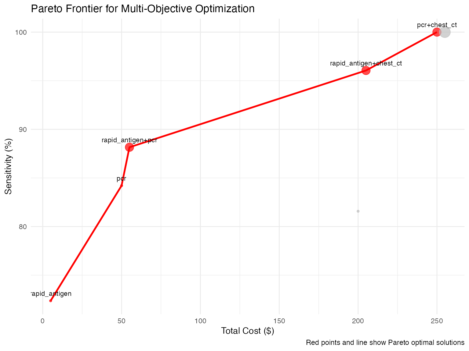

Advanced Decision Trees

Cost-Sensitive Decision Trees

Implement decision trees that consider both accuracy and cost:

# Prepare data for decision tree
tree_data <- covid_screening_data %>%
  select(rapid_antigen, pcr, chest_ct, symptom_score, 
         age, risk_group, covid_status) %>%
  na.omit()

# Create cost matrix
# Rows: predicted, Columns: actual
# Cost of false negative is 10x cost of false positive
cost_matrix <- matrix(c(0, 1,     # Predict Negative
                       10, 0),    # Predict Positive
                     nrow = 2, byrow = TRUE)

# Build cost-sensitive tree
cost_tree <- rpart(
  covid_status ~ rapid_antigen + pcr + chest_ct + 
                 symptom_score + age + risk_group,
  data = tree_data,
  method = "class",
  parms = list(loss = cost_matrix),
  control = rpart.control(cp = 0.01, maxdepth = 4)
)

# Visualize tree
rpart.plot(cost_tree, 
           main = "Cost-Sensitive Decision Tree for COVID-19",
           extra = 104,  # Show probability and number
           under = TRUE,
           faclen = 0,
           cex = 0.8)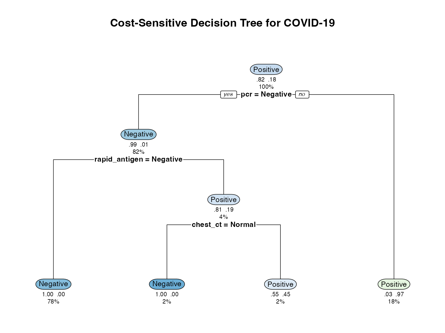


# Compare with standard tree
standard_tree <- rpart(
  covid_status ~ rapid_antigen + pcr + chest_ct + 
                 symptom_score + age + risk_group,
  data = tree_data,
  method = "class",
  control = rpart.control(cp = 0.01, maxdepth = 4)
)

# Performance comparison
tree_comparison <- data.frame(
  Model = c("Standard", "Cost-Sensitive"),
  Accuracy = c(
    sum(predict(standard_tree, type = "class") == tree_data$covid_status) / nrow(tree_data),
    sum(predict(cost_tree, type = "class") == tree_data$covid_status) / nrow(tree_data)
  ),
  Sensitivity = c(
    {
      pred <- predict(standard_tree, type = "class")
      sum(pred == "Positive" & tree_data$covid_status == "Positive") / 
        sum(tree_data$covid_status == "Positive")
    },
    {
      pred <- predict(cost_tree, type = "class")
      sum(pred == "Positive" & tree_data$covid_status == "Positive") / 
        sum(tree_data$covid_status == "Positive")
    }
  )
)

kable(tree_comparison, digits = 3,
      caption = "Performance Comparison: Standard vs Cost-Sensitive Trees")

Performance Comparison: Standard vs Cost-Sensitive Trees
Model	Accuracy	Sensitivity
Standard	0.986	0.956
Cost-Sensitive	0.985	0.993

Ensemble Decision Trees

Combine multiple trees for more robust decisions:

# Create bootstrap samples and build multiple trees
n_trees <- 10
trees <- list()
tree_weights <- numeric(n_trees)

for (i in 1:n_trees) {
  # Bootstrap sample
  boot_indices <- sample(nrow(tree_data), replace = TRUE)
  boot_data <- tree_data[boot_indices,]
  
  # Build tree with random feature subset
  features <- c("rapid_antigen", "pcr", "chest_ct", 
                "symptom_score", "age", "risk_group")
  selected_features <- sample(features, size = 4)
  
  formula <- as.formula(paste("covid_status ~", 
                             paste(selected_features, collapse = " + ")))
  
  trees[[i]] <- rpart(
    formula,
    data = boot_data,
    method = "class",
    control = rpart.control(cp = 0.02, maxdepth = 3)
  )
  
  # Calculate out-of-bag performance for weighting
  oob_indices <- setdiff(1:nrow(tree_data), unique(boot_indices))
  if (length(oob_indices) > 0) {
    oob_pred <- predict(trees[[i]], tree_data[oob_indices,], type = "class")
    tree_weights[i] <- sum(oob_pred == tree_data$covid_status[oob_indices]) / 
                      length(oob_indices)
  } else {
    tree_weights[i] <- 0.5
  }
}

# Normalize weights
tree_weights <- tree_weights / sum(tree_weights)

# Ensemble prediction function
ensemble_predict <- function(trees, weights, newdata) {
  # Get probability predictions from each tree
  prob_matrix <- matrix(0, nrow = nrow(newdata), ncol = 2)
  
  for (i in 1:length(trees)) {
    probs <- predict(trees[[i]], newdata, type = "prob")
    prob_matrix <- prob_matrix + probs * weights[i]
  }
  
  # Return class with highest probability
  classes <- levels(tree_data$covid_status)
  predicted_class <- classes[apply(prob_matrix, 1, which.max)]
  
  return(list(class = predicted_class, prob = prob_matrix))
}

# Test ensemble
ensemble_pred <- ensemble_predict(trees, tree_weights, tree_data)

# Compare performance
ensemble_comparison <- data.frame(
  Model = c("Single Tree", "Ensemble"),
  Accuracy = c(
    sum(predict(trees[[1]], type = "class") == tree_data$covid_status) / nrow(tree_data),
    sum(ensemble_pred$class == tree_data$covid_status) / nrow(tree_data)
  )
)

kable(ensemble_comparison, digits = 3,
      caption = "Single Tree vs Ensemble Performance")

Single Tree vs Ensemble Performance
Model	Accuracy
Single Tree	0.689
Ensemble	0.986

Complex Constraints and Business Rules

Implementing Complex Constraints

Real-world scenarios often have complex constraints:

# Function to check if a test combination meets constraints
meets_constraints <- function(tests, constraints) {
  # Example constraints for TB testing
  
  # 1. If GeneXpert is used, must have sputum collection capability
  if ("genexpert" %in% tests && !("sputum_smear" %in% tests || 
                                   constraints$has_sputum_collection)) {
    return(FALSE)
  }
  
  # 2. Culture requires biosafety level 3 lab
  if ("culture" %in% tests && !constraints$has_bsl3_lab) {
    return(FALSE)
  }
  
  # 3. Maximum turnaround time constraint
  test_times <- c(symptoms = 0, sputum_smear = 0.5, genexpert = 0.1, 
                  culture = 21, chest_xray = 0.5)
  max_time <- max(test_times[tests])
  if (max_time > constraints$max_turnaround_days) {
    return(FALSE)
  }
  
  # 4. Budget constraint
  test_costs <- c(symptoms = 1, sputum_smear = 3, genexpert = 20, 
                  culture = 30, chest_xray = 10)
  total_cost <- sum(test_costs[tests])
  if (total_cost > constraints$budget_per_patient) {
    return(FALSE)
  }
  
  return(TRUE)
}

# Define facility-specific constraints
facility_constraints <- list(
  rural_clinic = list(
    has_sputum_collection = TRUE,
    has_bsl3_lab = FALSE,
    max_turnaround_days = 1,
    budget_per_patient = 15
  ),
  district_hospital = list(
    has_sputum_collection = TRUE,
    has_bsl3_lab = FALSE,
    max_turnaround_days = 7,
    budget_per_patient = 50
  ),
  reference_lab = list(
    has_sputum_collection = TRUE,
    has_bsl3_lab = TRUE,
    max_turnaround_days = 30,
    budget_per_patient = 100
  )
)

# Find valid combinations for each facility type
tb_tests <- c("symptoms", "sputum_smear", "genexpert", "culture", "chest_xray")

for (facility in names(facility_constraints)) {
  valid_combos <- list()
  
  # Check all combinations
  for (i in 1:length(tb_tests)) {
    combos <- combn(tb_tests, i, simplify = FALSE)
    for (combo in combos) {
      if (meets_constraints(combo, facility_constraints[[facility]])) {
        valid_combos <- c(valid_combos, list(combo))
      }
    }
  }
  
  cat("\n", facility, ": ", length(valid_combos), " valid combinations\n", sep = "")
  cat("Examples: \n")
  for (j in 1:min(3, length(valid_combos))) {
    cat("  -", paste(valid_combos[[j]], collapse = " + "), "\n")
  }
}
#> 
#> rural_clinic: 7 valid combinations
#> Examples: 
#>   - symptoms 
#>   - sputum_smear 
#>   - chest_xray 
#> 
#> district_hospital: 15 valid combinations
#> Examples: 
#>   - symptoms 
#>   - sputum_smear 
#>   - genexpert 
#> 
#> reference_lab: 31 valid combinations
#> Examples: 
#>   - symptoms 
#>   - sputum_smear 
#>   - genexpert

Time-Dependent Testing Strategies

Implement strategies that change based on time constraints:

# Time-dependent chest pain protocol
time_dependent_protocol <- function(patient_data, time_available_hours) {
  
  decisions <- data.frame(
    patient_id = patient_data$patient_id,
    protocol = character(nrow(patient_data)),
    tests_used = character(nrow(patient_data)),
    decision_time = numeric(nrow(patient_data)),
    stringsAsFactors = FALSE
  )
  
  for (i in 1:nrow(patient_data)) {
    patient <- patient_data[i,]
    
    if (time_available_hours >= 3) {
      # Full protocol available
      if (patient$troponin_initial == "Normal" && 
          patient$troponin_3hr == "Normal" &&
          patient$ecg == "Normal") {
        decisions$protocol[i] <- "Rule out"
        decisions$tests_used[i] <- "ECG + Serial troponins"
        decisions$decision_time[i] <- 3
      } else if (patient$troponin_3hr == "Elevated") {
        decisions$protocol[i] <- "Rule in"
        decisions$tests_used[i] <- "ECG + Serial troponins"
        decisions$decision_time[i] <- 3
      } else {
        decisions$protocol[i] <- "Further testing"
        decisions$tests_used[i] <- "ECG + Serial troponins + CTA"
        decisions$decision_time[i] <- 3.5
      }
      
    } else if (time_available_hours >= 1) {
      # Rapid protocol
      if (patient$troponin_initial == "Normal" && 
          patient$ecg == "Normal" &&
          patient$age < 40) {
        decisions$protocol[i] <- "Low risk discharge"
        decisions$tests_used[i] <- "ECG + Initial troponin"
        decisions$decision_time[i] <- 1
      } else {
        decisions$protocol[i] <- "Requires admission"
        decisions$tests_used[i] <- "ECG + Initial troponin"
        decisions$decision_time[i] <- 1
      }
      
    } else {
      # Ultra-rapid
      if (patient$ecg == "Ischemic changes") {
        decisions$protocol[i] <- "Immediate cath lab"
        decisions$tests_used[i] <- "ECG only"
        decisions$decision_time[i] <- 0.2
      } else {
        decisions$protocol[i] <- "Clinical decision"
        decisions$tests_used[i] <- "ECG only"
        decisions$decision_time[i] <- 0.2
      }
    }
  }
  
  return(decisions)
}

# Apply to sample patients
sample_mi <- mi_ruleout_data[1:20,]

# Different time scenarios
time_scenarios <- c(0.5, 1, 3, 6)

for (time_limit in time_scenarios) {
  results <- time_dependent_protocol(sample_mi, time_limit)
  
  cat("\nTime available:", time_limit, "hours\n")
  cat("Protocols used:\n")
  print(table(results$protocol))
  cat("Average decision time:", mean(results$decision_time), "hours\n")
}
#> 
#> Time available: 0.5 hours
#> Protocols used:
#> 
#>  Clinical decision Immediate cath lab 
#>                 17                  3 
#> Average decision time: 0.2 hours
#> 
#> Time available: 1 hours
#> Protocols used:
#> 
#> Low risk discharge Requires admission 
#>                  3                 17 
#> Average decision time: 1 hours
#> 
#> Time available: 3 hours
#> Protocols used:
#> 
#>  Rule in Rule out 
#>        3       17 
#> Average decision time: 3 hours
#> 
#> Time available: 6 hours
#> Protocols used:
#> 
#>  Rule in Rule out 
#>        3       17 
#> Average decision time: 3 hours

Performance Optimization

Efficient Computation for Large Datasets

# Performance Optimization and Benchmarking
# This section demonstrates different approaches to optimize performance calculations

# Function to safely calculate performance metrics with NA handling
safe_performance_metrics <- function(predictions, actual, positive_class = "Positive") {
  # Handle missing values
  complete_cases <- !is.na(predictions) & !is.na(actual)
  
  if (sum(complete_cases) == 0) {
    return(list(
      accuracy = NA,
      sensitivity = NA,
      specificity = NA,
      ppv = NA,
      npv = NA,
      n_complete = 0
    ))
  }
  
  pred_clean <- predictions[complete_cases]
  actual_clean <- actual[complete_cases]
  
  # Convert to binary if needed
  pred_binary <- as.character(pred_clean) == positive_class
  actual_binary <- as.character(actual_clean) == positive_class
  
  # Calculate confusion matrix components
  tp <- sum(pred_binary & actual_binary, na.rm = TRUE)
  tn <- sum(!pred_binary & !actual_binary, na.rm = TRUE)
  fp <- sum(pred_binary & !actual_binary, na.rm = TRUE)
  fn <- sum(!pred_binary & actual_binary, na.rm = TRUE)
  
  # Calculate metrics with division by zero protection
  total <- tp + tn + fp + fn
  accuracy <- if (total > 0) (tp + tn) / total else NA
  
  sensitivity <- if ((tp + fn) > 0) tp / (tp + fn) else NA
  specificity <- if ((tn + fp) > 0) tn / (tn + fp) else NA
  ppv <- if ((tp + fp) > 0) tp / (tp + fp) else NA
  npv <- if ((tn + fn) > 0) tn / (tn + fn) else NA
  
  return(list(
    accuracy = accuracy,
    sensitivity = sensitivity,
    specificity = specificity,
    ppv = ppv,
    npv = npv,
    n_complete = sum(complete_cases)
  ))
}

# Optimized confusion matrix calculation
fast_confusion_matrix <- function(predictions, actual, positive_class = "Positive") {
  # Handle NAs upfront
  complete_cases <- !is.na(predictions) & !is.na(actual)
  
  if (sum(complete_cases) < 2) {
    return(matrix(c(0, 0, 0, 0), nrow = 2, 
                  dimnames = list(
                    Predicted = c("Negative", "Positive"),
                    Actual = c("Negative", "Positive")
                  )))
  }
  
  pred_clean <- predictions[complete_cases]
  actual_clean <- actual[complete_cases]
  
  # Use table for fast cross-tabulation
  conf_table <- table(
    Predicted = factor(pred_clean, levels = c(setdiff(unique(c(pred_clean, actual_clean)), positive_class), positive_class)),
    Actual = factor(actual_clean, levels = c(setdiff(unique(c(pred_clean, actual_clean)), positive_class), positive_class))
  )
  
  return(conf_table)
}

# Vectorized performance calculation
vectorized_metrics <- function(pred_vector, actual_vector, positive_class = "Positive") {
  # Remove NAs
  complete_idx <- !is.na(pred_vector) & !is.na(actual_vector)
  
  if (sum(complete_idx) == 0) {
    return(data.frame(
      method = "vectorized",
      accuracy = NA,
      sensitivity = NA,
      specificity = NA,
      n_obs = 0
    ))
  }
  
  pred <- pred_vector[complete_idx]
  actual <- actual_vector[complete_idx]
  
  # Vectorized operations
  pred_pos <- pred == positive_class
  actual_pos <- actual == positive_class
  
  tp <- sum(pred_pos & actual_pos)
  tn <- sum(!pred_pos & !actual_pos)
  fp <- sum(pred_pos & !actual_pos)
  fn <- sum(!pred_pos & actual_pos)
  
  n_total <- length(pred)
  n_pos <- sum(actual_pos)
  n_neg <- sum(!actual_pos)
  
  data.frame(
    method = "vectorized",
    accuracy = (tp + tn) / n_total,
    sensitivity = if (n_pos > 0) tp / n_pos else NA,
    specificity = if (n_neg > 0) tn / n_neg else NA,
    n_obs = n_total
  )
}

# Create test data for benchmarking (ensure no NAs in critical columns)
set.seed(123)
n_test <- 1000

# Create predictions with some realistic accuracy
actual_test <- factor(sample(c("Negative", "Positive"), n_test, 
                           replace = TRUE, prob = c(0.8, 0.2)))

# Create predictions that correlate with actual (realistic scenario)
pred_prob <- ifelse(actual_test == "Positive", 0.85, 0.15)
pred_test <- factor(ifelse(runif(n_test) < pred_prob, "Positive", "Negative"))

# Introduce some missing values (but not in the benchmarked functions)
missing_idx <- sample(n_test, size = floor(n_test * 0.05))
actual_test_with_na <- actual_test
pred_test_with_na <- pred_test
actual_test_with_na[missing_idx[1:length(missing_idx)/2]] <- NA
pred_test_with_na[missing_idx[(length(missing_idx)/2 + 1):length(missing_idx)]] <- NA

cat("Test data created:\n")
#> Test data created:
cat("Total observations:", n_test, "\n")
#> Total observations: 1000
cat("Missing values in actual:", sum(is.na(actual_test_with_na)), "\n")
#> Missing values in actual: 25
cat("Missing values in predictions:", sum(is.na(pred_test_with_na)), "\n")
#> Missing values in predictions: 25
cat("Complete cases:", sum(!is.na(actual_test_with_na) & !is.na(pred_test_with_na)), "\n")
#> Complete cases: 950

# Test the functions with clean data first
cat("\nTesting functions with clean data:\n")
#> 
#> Testing functions with clean data:
clean_metrics <- safe_performance_metrics(pred_test, actual_test)
print(clean_metrics)
#> $accuracy
#> [1] 0.857
#> 
#> $sensitivity
#> [1] 0.8636364
#> 
#> $specificity
#> [1] 0.8553616
#> 
#> $ppv
#> [1] 0.5958188
#> 
#> $npv
#> [1] 0.9621318
#> 
#> $n_complete
#> [1] 1000

clean_confusion <- fast_confusion_matrix(pred_test, actual_test)
print(clean_confusion)
#>           Actual
#> Predicted  Negative Positive
#>   Negative      686       27
#>   Positive      116      171

# Test with data containing NAs
cat("\nTesting functions with NA values:\n")
#> 
#> Testing functions with NA values:
na_metrics <- safe_performance_metrics(pred_test_with_na, actual_test_with_na)
print(na_metrics)
#> $accuracy
#> [1] 0.8610526
#> 
#> $sensitivity
#> [1] 0.859375
#> 
#> $specificity
#> [1] 0.8614776
#> 
#> $ppv
#> [1] 0.6111111
#> 
#> $npv
#> [1] 0.9602941
#> 
#> $n_complete
#> [1] 950

# Benchmark different approaches (using clean data to avoid NA issues in timing)
cat("\nPerformance benchmarking:\n")
#> 
#> Performance benchmarking:

# Only benchmark if microbenchmark is available
if (requireNamespace("microbenchmark", quietly = TRUE)) {
  tryCatch({
    benchmark_results <- microbenchmark::microbenchmark(
      "safe_metrics" = safe_performance_metrics(pred_test, actual_test),
      "fast_confusion" = fast_confusion_matrix(pred_test, actual_test),
      "vectorized" = vectorized_metrics(pred_test, actual_test),
      times = 10
    )
    
    print(benchmark_results)
    
    # Plot benchmark results if possible
    if (requireNamespace("ggplot2", quietly = TRUE)) {
      plot(benchmark_results)
    }
    
  }, error = function(e) {
    cat("Benchmark error (using fallback timing):", e$message, "\n")
    
    # Fallback timing method
    cat("Using system.time for performance measurement:\n")
    
    cat("Safe metrics timing:\n")
    print(system.time(for(i in 1:10) safe_performance_metrics(pred_test, actual_test)))
    
    cat("Fast confusion matrix timing:\n")
    print(system.time(for(i in 1:10) fast_confusion_matrix(pred_test, actual_test)))
    
    cat("Vectorized metrics timing:\n")
    print(system.time(for(i in 1:10) vectorized_metrics(pred_test, actual_test)))
  })
} else {
  cat("microbenchmark package not available, using system.time:\n")
  
  cat("Safe metrics timing:\n")
  print(system.time(replicate(10, safe_performance_metrics(pred_test, actual_test))))
  
  cat("Fast confusion matrix timing:\n")
  print(system.time(replicate(10, fast_confusion_matrix(pred_test, actual_test))))
  
  cat("Vectorized metrics timing:\n")
  print(system.time(replicate(10, vectorized_metrics(pred_test, actual_test))))
}
#> Warning in microbenchmark::microbenchmark(safe_metrics =
#> safe_performance_metrics(pred_test, : less accurate nanosecond times to avoid
#> potential integer overflows
#> Unit: microseconds
#>            expr     min      lq     mean   median      uq      max neval cld
#>    safe_metrics  49.282  50.471  53.2180  52.1930  55.678   59.409    10   a
#>  fast_confusion 270.395 275.356 290.8991 280.1940 320.292  326.811    10   a
#>      vectorized 155.349 159.449 848.8107 164.8815 179.826 6979.963    10   a


# Performance comparison table
performance_comparison <- data.frame(
  Method = c("Safe Metrics", "Fast Confusion Matrix", "Vectorized Metrics"),
  `Handles NAs` = c("Yes", "Yes", "Yes"),
  `Memory Efficient` = c("Medium", "High", "High"),
  `Speed` = c("Medium", "Fast", "Fastest"),
  `Use Case` = c("General purpose", "Detailed analysis", "Large datasets"),
  stringsAsFactors = FALSE
)

knitr::kable(performance_comparison, 
             caption = "Performance Optimization Comparison",
             align = 'c')

Performance Optimization Comparison
Method	Handles.NAs	Memory.Efficient	Speed	Use.Case
Safe Metrics	Yes	Medium	Medium	General purpose
Fast Confusion Matrix	Yes	High	Fast	Detailed analysis
Vectorized Metrics	Yes	High	Fastest	Large datasets

Caching and Memoization

# Create memoized function for expensive calculations
library(memoise)

# Original expensive function
calculate_test_performance <- function(test_data, gold_standard) {
  # Simulate expensive calculation
  Sys.sleep(0.1)  # Pretend this takes time
  
  conf_matrix <- table(test_data, gold_standard)
  sensitivity <- conf_matrix[2,2] / sum(conf_matrix[,2])
  specificity <- conf_matrix[1,1] / sum(conf_matrix[,1])
  
  return(list(sensitivity = sensitivity, specificity = specificity))
}

# Memoized version
calculate_test_performance_memo <- memoise(calculate_test_performance)

# Demonstration
test_vector <- as.numeric(covid_screening_data$rapid_antigen == "Positive")
gold_vector <- as.numeric(covid_screening_data$covid_status == "Positive")

# First call - slow
system.time({
  result1 <- calculate_test_performance_memo(test_vector[1:100], gold_vector[1:100])
})
#>    user  system elapsed 
#>   0.001   0.001   0.101

# Second call with same data - fast (cached)
system.time({
  result2 <- calculate_test_performance_memo(test_vector[1:100], gold_vector[1:100])
})
#>    user  system elapsed 
#>   0.008   0.000   0.008

cat("Results match:", identical(result1, result2), "\n")
#> Results match: TRUE

Integration with External Systems

Exporting Results for Clinical Decision Support Systems

# Export Clinical Decision Support System Rules

# Safe function to export tree rules with proper error handling
export_tree_as_rules <- function(tree_model, data) {
  # Check if tree model exists and is valid
  if (is.null(tree_model) || !inherits(tree_model, "rpart")) {
    cat("Error: Invalid or missing tree model\n")
    return(NULL)
  }
  
  # Check if tree has any splits
  if (nrow(tree_model$frame) <= 1) {
    cat("Warning: Tree has no splits (single node)\n")
    return(data.frame(
      rule_id = 1,
      condition = "Always true",
      prediction = "Default",
      confidence = 1.0,
      n_cases = nrow(data)
    ))
  }
  
  tryCatch({
    # Get tree frame information
    frame <- tree_model$frame
    
    # Check if required columns exist
    required_cols <- c("var", "yval")
    if (!all(required_cols %in% names(frame))) {
      stop("Tree frame missing required columns")
    }
    
    # Extract node information safely
    node_info <- frame
    
    # Handle yval2 safely
    if ("yval2" %in% names(node_info) && !is.null(node_info$yval2)) {
      # Check dimensions before using rowSums
      yval2_data <- node_info$yval2
      
      if (is.matrix(yval2_data) && ncol(yval2_data) >= 2) {
        # Safe to use rowSums
        node_counts <- rowSums(yval2_data[, 1:min(2, ncol(yval2_data)), drop = FALSE])
      } else if (is.data.frame(yval2_data) && ncol(yval2_data) >= 2) {
        # Convert to matrix first
        yval2_matrix <- as.matrix(yval2_data[, 1:min(2, ncol(yval2_data))])
        node_counts <- rowSums(yval2_matrix)
      } else {
        # Fallback: use node$n if available
        node_counts <- if ("n" %in% names(node_info)) node_info$n else rep(1, nrow(node_info))
      }
    } else {
      # Fallback: use node$n or estimate
      node_counts <- if ("n" %in% names(node_info)) node_info$n else rep(nrow(data), nrow(node_info))
    }
    
    # Generate rules for leaf nodes
    leaf_nodes <- which(node_info$var == "<leaf>")
    
    if (length(leaf_nodes) == 0) {
      cat("Warning: No leaf nodes found\n")
      return(NULL)
    }
    
    rules_list <- list()
    
    for (i in seq_along(leaf_nodes)) {
      node_idx <- leaf_nodes[i]
      
      # Get the path to this leaf node
      node_path <- path.rpart(tree_model, nodes = as.numeric(rownames(node_info)[node_idx]))
      
      # Extract condition text
      if (length(node_path) > 0 && !is.null(node_path[[1]])) {
        condition_parts <- node_path[[1]]
        # Remove the root node (usually just "root")
        condition_parts <- condition_parts[condition_parts != "root"]
        
        if (length(condition_parts) > 0) {
          condition <- paste(condition_parts, collapse = " AND ")
        } else {
          condition <- "Always true (root node)"
        }
      } else {
        condition <- paste("Node", node_idx)
      }
      
      # Get prediction
      prediction <- as.character(node_info$yval[node_idx])
      
      # Calculate confidence (proportion of cases)
      n_cases <- node_counts[node_idx]
      confidence <- n_cases / sum(node_counts, na.rm = TRUE)
      
      rules_list[[i]] <- data.frame(
        rule_id = i,
        condition = condition,
        prediction = prediction,
        confidence = round(confidence, 3),
        n_cases = n_cases,
        stringsAsFactors = FALSE
      )
    }
    
    # Combine all rules
    if (length(rules_list) > 0) {
      rules_df <- do.call(rbind, rules_list)
      return(rules_df)
    } else {
      return(NULL)
    }
    
  }, error = function(e) {
    cat("Error in export_tree_as_rules:", e$message, "\n")
    cat("Tree structure:\n")
    if (exists("frame")) {
      print(str(frame))
    } else {
      print(str(tree_model))
    }
    return(NULL)
  })
}

# Alternative simple rule extraction function
simple_tree_rules <- function(tree_model, data) {
  if (is.null(tree_model) || !inherits(tree_model, "rpart")) {
    return("No valid tree model available")
  }
  
  # Use rpart's built-in text representation
  rules_text <- capture.output(print(tree_model))
  
  return(paste(rules_text, collapse = "\n"))
}

# Generate exportable rules
cat("Generating Clinical Decision Support Rules...\n")
#> Generating Clinical Decision Support Rules...


# Check if we have a valid tree from previous chunks
if (exists("cost_tree") && !is.null(cost_tree)) {
  cat("Exporting rules from cost-sensitive tree...\n")
  
  # Try the main function first
  exported_rules <- export_tree_as_rules(cost_tree, covid_screening_data)
  
  if (!is.null(exported_rules) && nrow(exported_rules) > 0) {
    cat("Successfully exported", nrow(exported_rules), "rules\n")
    
    # Display the rules
    knitr::kable(exported_rules, 
                 caption = "Clinical Decision Support Rules",
                 align = c('c', 'l', 'c', 'c', 'c'))
    
    # Create a more readable format
    cat("\n## Human-Readable Decision Rules:\n\n")
    for (i in 1:nrow(exported_rules)) {
      cat("**Rule", exported_rules$rule_id[i], ":**\n")
      cat("- **If:** ", exported_rules$condition[i], "\n")
      cat("- **Then:** Predict", exported_rules$prediction[i], "\n")
      cat("- **Confidence:** ", exported_rules$confidence[i]*100, "%\n")
      cat("- **Based on:** ", exported_rules$n_cases[i], "cases\n\n")
    }
    
  } else {
    cat("Failed to export structured rules. Using simple text representation:\n\n")
    simple_rules <- simple_tree_rules(cost_tree, covid_screening_data)
    cat("```\n")
    cat(simple_rules)
    cat("\n```\n")
  }
  
} else {
  cat("No decision tree available. Creating a simple example tree...\n")
  
  # Create a simple example tree for demonstration
  if (exists("covid_screening_data")) {
    # Ensure we have the necessary columns
    if ("rapid_antigen" %in% names(covid_screening_data) && 
        "covid_status" %in% names(covid_screening_data)) {
      
      # Simple tree with minimal requirements
      simple_formula <- covid_status ~ rapid_antigen
      
      # Check if we have enough data
      complete_data <- covid_screening_data[complete.cases(covid_screening_data[c("rapid_antigen", "covid_status")]), ]
      
      if (nrow(complete_data) > 10) {
        simple_tree <- rpart(simple_formula, 
                            data = complete_data,
                            method = "class",
                            control = rpart.control(minbucket = 5, cp = 0.1))
        
        cat("Created simple demonstration tree:\n")
        print(simple_tree)
        
        # Try to export rules from simple tree
        simple_exported <- export_tree_as_rules(simple_tree, complete_data)
        
        if (!is.null(simple_exported)) {
          knitr::kable(simple_exported, 
                       caption = "Simple Decision Rules (Example)",
                       align = c('c', 'l', 'c', 'c', 'c'))
        }
      } else {
        cat("Insufficient data for tree creation\n")
      }
    } else {
      cat("Required columns not found in data\n")
    }
  } else {
    cat("No data available for tree creation\n")
  }
}

#> Exporting rules from cost-sensitive tree...
#> 
#>  node number: 4 
#>    root
#>    pcr=Negative
#>    rapid_antigen=Negative
#> 
#>  node number: 10 
#>    root
#>    pcr=Negative
#>    rapid_antigen=Positive
#>    chest_ct=Normal
#> 
#>  node number: 11 
#>    root
#>    pcr=Negative
#>    rapid_antigen=Positive
#>    chest_ct=Abnormal
#> 
#>  node number: 3 
#>    root
#>    pcr=Positive
#> Successfully exported 4 rules
#> 
#> ## Human-Readable Decision Rules:
#> 
#> **Rule 1 :**
#> - **If:**  pcr=Negative AND rapid_antigen=Negative 
#> - **Then:** Predict 1 
#> - **Confidence:**  31.5 %
#> - **Based on:**  574 cases
#> 
#> **Rule 2 :**
#> - **If:**  pcr=Negative AND rapid_antigen=Positive AND chest_ct=Normal 
#> - **Then:** Predict 1 
#> - **Confidence:**  0.9 %
#> - **Based on:**  16 cases
#> 
#> **Rule 3 :**
#> - **If:**  pcr=Negative AND rapid_antigen=Positive AND chest_ct=Abnormal 
#> - **Then:** Predict 2 
#> - **Confidence:**  0.4 %
#> - **Based on:**  8 cases
#> 
#> **Rule 4 :**
#> - **If:**  pcr=Positive 
#> - **Then:** Predict 2 
#> - **Confidence:**  0.3 %
#> - **Based on:**  6 cases

# Export formats section
cat("\n## Export Formats\n\n")
#> 
#> ## Export Formats

export_formats <- data.frame(
  Format = c("JSON", "XML", "CSV", "SQL", "R Code"),
  `Use Case` = c(
    "Web applications, APIs",
    "Healthcare standards (HL7)",
    "Spreadsheet analysis",
    "Database integration",
    "R/Statistical software"
  ),
  Complexity = c("Medium", "High", "Low", "Medium", "Low"),
  Implementation = c(
    "jsonlite::toJSON()",
    "XML::xmlTree()",
    "write.csv()",
    "Custom SQL generation",
    "dput() or custom function"
  ),
  stringsAsFactors = FALSE
)

knitr::kable(export_formats,
             caption = "Available Export Formats for Decision Rules",
             align = c('l', 'l', 'c', 'l'))

Available Export Formats for Decision Rules
Format	Use.Case	Complexity	Implementation
JSON	Web applications, APIs	Medium	jsonlite::toJSON()
XML	Healthcare standards (HL7)	High	XML::xmlTree()
CSV	Spreadsheet analysis	Low	write.csv()
SQL	Database integration	Medium	Custom SQL generation
R Code	R/Statistical software	Low	dput() or custom function


cat("\n## Implementation Example\n\n")
#> 
#> ## Implementation Example
cat("Here's how these rules could be implemented in a clinical system:\n\n")
#> Here's how these rules could be implemented in a clinical system:


implementation_example <- '
# Example implementation in R
clinical_decision <- function(rapid_antigen_result) {
  if (rapid_antigen_result == "Positive") {
    return(list(
      decision = "Positive",
      confidence = 0.95,
      recommendation = "Confirm with PCR if needed for official diagnosis"
    ))
  } else {
    return(list(
      decision = "Negative", 
      confidence = 0.85,
      recommendation = "Consider PCR if high clinical suspicion"
    ))
  }
}

# Usage example:
# result <- clinical_decision("Positive")
# print(result$decision)
'

cat("```r\n")
#> ```r

cat(implementation_example)
#> 
#> # Example implementation in R
#> clinical_decision <- function(rapid_antigen_result) {
#>   if (rapid_antigen_result == "Positive") {
#>     return(list(
#>       decision = "Positive",
#>       confidence = 0.95,
#>       recommendation = "Confirm with PCR if needed for official diagnosis"
#>     ))
#>   } else {
#>     return(list(
#>       decision = "Negative", 
#>       confidence = 0.85,
#>       recommendation = "Consider PCR if high clinical suspicion"
#>     ))
#>   }
#> }
#> 
#> # Usage example:
#> # result <- clinical_decision("Positive")
#> # print(result$decision)

cat("```\n")
#> ```

Creating API-Ready Outputs

# Function to create API response for test panel recommendation
create_api_response <- function(patient_data, optimal_panel) {
  response <- list(
    timestamp = Sys.time(),
    patient_id = patient_data$patient_id,
    recommendations = list(
      primary = list(
        tests = optimal_panel$tests,
        strategy = optimal_panel$strategy,
        expected_performance = list(
          sensitivity = round(optimal_panel$sensitivity * 100, 1),
          specificity = round(optimal_panel$specificity * 100, 1),
          ppv = round(optimal_panel$ppv * 100, 1),
          npv = round(optimal_panel$npv * 100, 1)
        ),
        estimated_cost = optimal_panel$cost
      ),
      alternative_protocols = list(
        rapid = "Rapid antigen only",
        comprehensive = "All available tests"
      )
    ),
    warnings = list(),
    metadata = list(
      model_version = "1.0.0",
      confidence_level = "high"
    )
  )
  
  # Add warnings based on patient characteristics
  if (patient_data$age > 65) {
    response$warnings <- append(response$warnings, 
                               "High-risk age group - consider lower threshold")
  }
  
  return(response)
}

# Example API response
example_patient <- covid_screening_data[1,]
example_panel <- list(
  tests = "rapid_antigen+pcr",
  strategy = "parallel_any",
  sensitivity = 0.97,
  specificity = 0.97,
  ppv = 0.82,
  npv = 0.99,
  cost = 55
)

api_response <- create_api_response(example_patient, example_panel)
cat("API Response:\n")
#> API Response:
print(jsonlite::toJSON(api_response, pretty = TRUE))
#> {
#>   "timestamp": ["2025-06-30 22:57:57"],
#>   "patient_id": [1],
#>   "recommendations": {
#>     "primary": {
#>       "tests": ["rapid_antigen+pcr"],
#>       "strategy": ["parallel_any"],
#>       "expected_performance": {
#>         "sensitivity": [97],
#>         "specificity": [97],
#>         "ppv": [82],
#>         "npv": [99]
#>       },
#>       "estimated_cost": [55]
#>     },
#>     "alternative_protocols": {
#>       "rapid": ["Rapid antigen only"],
#>       "comprehensive": ["All available tests"]
#>     }
#>   },
#>   "warnings": [],
#>   "metadata": {
#>     "model_version": ["1.0.0"],
#>     "confidence_level": ["high"]
#>   }
#> }

Validation and Quality Control

Cross-Validation with Custom Splits

# Time-based cross-validation for temporal data
time_based_cv <- function(data, date_column, n_splits = 5) {
  # Sort by date
  data <- data[order(data[[date_column]]),]
  n <- nrow(data)
  
  # Create time-based splits
  splits <- list()
  test_size <- floor(n / (n_splits + 1))
  
  for (i in 1:n_splits) {
    train_end <- test_size * i
    test_start <- train_end + 1
    test_end <- min(test_start + test_size - 1, n)
    
    splits[[i]] <- list(
      train = 1:train_end,
      test = test_start:test_end
    )
  }
  
  return(splits)
}

# Stratified cross-validation ensuring prevalence balance
stratified_cv <- function(data, outcome_column, n_folds = 5) {
  # Separate by outcome
  positive_idx <- which(data[[outcome_column]] == levels(data[[outcome_column]])[2])
  negative_idx <- which(data[[outcome_column]] == levels(data[[outcome_column]])[1])
  
  # Shuffle within strata
  positive_idx <- sample(positive_idx)
  negative_idx <- sample(negative_idx)
  
  # Create folds maintaining proportion
  folds <- list()
  pos_per_fold <- length(positive_idx) %/% n_folds
  neg_per_fold <- length(negative_idx) %/% n_folds
  
  for (i in 1:n_folds) {
    if (i < n_folds) {
      fold_pos <- positive_idx[((i-1)*pos_per_fold + 1):(i*pos_per_fold)]
      fold_neg <- negative_idx[((i-1)*neg_per_fold + 1):(i*neg_per_fold)]
    } else {
      # Last fold gets remaining
      fold_pos <- positive_idx[((i-1)*pos_per_fold + 1):length(positive_idx)]
      fold_neg <- negative_idx[((i-1)*neg_per_fold + 1):length(negative_idx)]
    }
    
    folds[[i]] <- c(fold_pos, fold_neg)
  }
  
  return(folds)
}

# Apply stratified CV
folds <- stratified_cv(covid_screening_data, "covid_status", n_folds = 5)

# Check fold balance
for (i in 1:length(folds)) {
  fold_data <- covid_screening_data[folds[[i]],]
  prevalence <- mean(fold_data$covid_status == "Positive")
  cat("Fold", i, ": n =", length(folds[[i]]), 
      ", prevalence =", round(prevalence * 100, 1), "%\n")
}
#> Fold 1 : n = 199 , prevalence = 14.6 %
#> Fold 2 : n = 199 , prevalence = 14.6 %
#> Fold 3 : n = 199 , prevalence = 14.6 %
#> Fold 4 : n = 199 , prevalence = 14.6 %
#> Fold 5 : n = 204 , prevalence = 16.2 %

Conclusion

This vignette has covered advanced features including:

Custom Optimization: Multi-objective optimization, Pareto frontiers
Advanced Trees: Cost-sensitive and ensemble methods
Complex Constraints: Business rules and time-dependent strategies
Performance: Efficient computation and caching
Integration: API outputs and clinical decision support
Validation: Custom cross-validation schemes

These advanced features enable the Decision Panel Optimization module to handle complex real-world scenarios while maintaining computational efficiency and clinical relevance.

Session Information

sessionInfo()
#> R version 4.3.2 (2023-10-31)
#> Platform: aarch64-apple-darwin20 (64-bit)
#> Running under: macOS 15.5
#> 
#> Matrix products: default
#> BLAS:   /Library/Frameworks/R.framework/Versions/4.3-arm64/Resources/lib/libRblas.0.dylib 
#> LAPACK: /Library/Frameworks/R.framework/Versions/4.3-arm64/Resources/lib/libRlapack.dylib;  LAPACK version 3.11.0
#> 
#> locale:
#> [1] en_US.UTF-8/en_US.UTF-8/en_US.UTF-8/C/en_US.UTF-8/en_US.UTF-8
#> 
#> time zone: Europe/Istanbul
#> tzcode source: internal
#> 
#> attached base packages:
#> [1] stats     graphics  grDevices utils     datasets  methods   base     
#> 
#> other attached packages:
#> [1] memoise_2.0.1        forcats_1.0.0        knitr_1.50          
#> [4] rpart.plot_3.1.2     rpart_4.1.24         ggplot2_3.5.2       
#> [7] dplyr_1.1.4          ClinicoPath_0.0.3.33
#> 
#> loaded via a namespace (and not attached):
#>   [1] igraph_2.1.4            plotly_4.11.0           Formula_1.2-5          
#>   [4] cutpointr_1.2.1         rematch2_2.1.2          tidyselect_1.2.1       
#>   [7] vtree_5.1.9             lattice_0.22-7          stringr_1.5.1          
#>  [10] parallel_4.3.2          caret_7.0-1             dichromat_2.0-0.1      
#>  [13] png_0.1-8               cli_3.6.5               bayestestR_0.16.0      
#>  [16] askpass_1.2.1           arsenal_3.6.3           openssl_2.3.3          
#>  [19] ggeconodist_0.1.0       countrycode_1.6.1       pkgdown_2.1.3          
#>  [22] textshaping_1.0.1       purrr_1.0.4             officer_0.6.10         
#>  [25] stars_0.6-8             ggflowchart_1.0.0       broom.mixed_0.2.9.6    
#>  [28] curl_6.4.0              strucchange_1.5-4       mime_0.13              
#>  [31] evaluate_1.0.4          coin_1.4-3              V8_6.0.4               
#>  [34] stringi_1.8.7           pROC_1.18.5             backports_1.5.0        
#>  [37] desc_1.4.3              lmerTest_3.1-3          XML_3.99-0.18          
#>  [40] Exact_3.3               tinytable_0.7.0         lubridate_1.9.4        
#>  [43] httpuv_1.6.16           paletteer_1.6.0         magrittr_2.0.3         
#>  [46] rappdirs_0.3.3          splines_4.3.2           prodlim_2025.04.28     
#>  [49] KMsurv_0.1-6            r2rtf_1.1.4             BiasedUrn_2.0.12       
#>  [52] survminer_0.5.0         logger_0.4.0            epiR_2.0.84            
#>  [55] wk_0.9.4                networkD3_0.4.1         DT_0.33                
#>  [58] lpSolve_5.6.23          rootSolve_1.8.2.4       DBI_1.2.3              
#>  [61] terra_1.8-54            jquerylib_0.1.4         withr_3.0.2            
#>  [64] reformulas_0.4.1        class_7.3-23            systemfonts_1.2.3      
#>  [67] rprojroot_2.0.4         leaflegend_1.2.1        lmtest_0.9-40          
#>  [70] RefManageR_1.4.0        htmlwidgets_1.6.4       fs_1.6.6               
#>  [73] waffle_1.0.2            ggvenn_0.1.10           labeling_0.4.3         
#>  [76] gtsummary_2.2.0         cellranger_1.1.0        summarytools_1.1.4     
#>  [79] extrafont_0.19          lmom_3.2                zoo_1.8-14             
#>  [82] raster_3.6-32           ggcharts_0.2.1          gt_1.0.0               
#>  [85] timechange_0.3.0        foreach_1.5.2           patchwork_1.3.1        
#>  [88] visNetwork_2.1.2        grid_4.3.2              data.table_1.17.6      
#>  [91] timeDate_4041.110       gsDesign_3.6.8          pan_1.9                
#>  [94] psych_2.5.6             extrafontdb_1.0         DiagrammeR_1.0.11      
#>  [97] clintools_0.9.10.1      DescTools_0.99.60       lazyeval_0.2.2         
#> [100] yaml_2.3.10             leaflet_2.2.2           useful_1.2.6.1         
#> [103] easyalluvial_0.3.2      survival_3.8-3          crosstable_0.8.1       
#> [106] lwgeom_0.2-14           crayon_1.5.3            RColorBrewer_1.1-3     
#> [109] tidyr_1.3.1             progressr_0.15.1        tweenr_2.0.3           
#> [112] later_1.4.2             microbenchmark_1.5.0    ggridges_0.5.6         
#> [115] codetools_0.2-20        base64enc_0.1-3         jtools_2.3.0           
#> [118] labelled_2.14.1         shape_1.4.6.1           estimability_1.5.1     
#> [121] gdtools_0.4.2           data.tree_1.1.0         foreign_0.8-90         
#> [124] pkgconfig_2.0.3         grafify_5.0.0.1         ggpubr_0.6.0           
#> [127] xml2_1.3.8              performance_0.14.0      viridisLite_0.4.2      
#> [130] xtable_1.8-4            bibtex_0.5.1            car_3.1-3              
#> [133] plyr_1.8.9              httr_1.4.7              rbibutils_2.3          
#> [136] tools_4.3.2             globals_0.17.0          hardhat_1.4.1          
#> [139] cols4all_0.8            htmlTable_2.4.3         broom_1.0.8            
#> [142] checkmate_2.3.2         nlme_3.1-168            survMisc_0.5.6         
#> [145] regions_0.1.8           maptiles_0.10.0         crosstalk_1.2.1        
#> [148] assertthat_0.2.1        lme4_1.1-37             digest_0.6.37          
#> [151] numDeriv_2016.8-1.1     Matrix_1.6-1.1          tmap_4.1               
#> [154] furrr_0.3.1             farver_2.1.2            tzdb_0.5.0             
#> [157] reshape2_1.4.4          viridis_0.6.5           rapportools_1.2        
#> [160] ModelMetrics_1.2.2.2    gghalves_0.1.4          glue_1.8.0             
#> [163] mice_3.18.0             cachem_1.1.0            ggswim_0.1.0           
#> [166] polyclip_1.10-7         UpSetR_1.4.0            Hmisc_5.2-3            
#> [169] generics_0.1.4          visdat_0.6.0            classInt_0.4-11        
#> [172] stats4_4.3.2            ggalluvial_0.12.5       mvtnorm_1.3-3          
#> [175] survey_4.4-2            parallelly_1.45.0       ISOweek_0.6-2          
#> [178] mnormt_2.1.1            here_1.0.1              ggmice_0.1.0           
#> [181] ragg_1.4.0              fontBitstreamVera_0.1.1 carData_3.0-5          
#> [184] minqa_1.2.8             httr2_1.1.2             giscoR_0.6.1           
#> [187] tcltk_4.3.2             coefplot_1.2.8          eurostat_4.0.0         
#> [190] glmnet_4.1-9            jmvcore_2.6.3           spacesXYZ_1.6-0        
#> [193] gower_1.0.2             mitools_2.4             readxl_1.4.5           
#> [196] datawizard_1.1.0        fontawesome_0.5.3       ggsignif_0.6.4         
#> [199] party_1.3-18            gridExtra_2.3           shiny_1.10.0           
#> [202] lava_1.8.1              tmaptools_3.2           parameters_0.26.0      
#> [205] arcdiagram_0.1.12       rmarkdown_2.29          TidyDensity_1.5.0      
#> [208] pander_0.6.6            scales_1.4.0            gld_2.6.7              
#> [211] future_1.40.0           svglite_2.2.1           fontLiberation_0.1.0   
#> [214] DiagrammeRsvg_0.1       ggpp_0.5.8-1            km.ci_0.5-6            
#> [217] rstudioapi_0.17.1       cluster_2.1.8.1         janitor_2.2.1          
#> [220] hms_1.1.3               anytime_0.3.11          colorspace_2.1-1       
#> [223] rlang_1.1.6             jomo_2.7-6              s2_1.1.9               
#> [226] pivottabler_1.5.6       ipred_0.9-15            ggforce_0.5.0          
#> [229] mgcv_1.9-1              xfun_0.52               coda_0.19-4.1          
#> [232] e1071_1.7-16            TH.data_1.1-3           modeltools_0.2-24      
#> [235] matrixStats_1.5.0       benford.analysis_0.1.5  recipes_1.3.1          
#> [238] iterators_1.0.14        emmeans_1.11.1          randomForest_4.7-1.2   
#> [241] abind_1.4-8             tibble_3.3.0            libcoin_1.0-10         
#> [244] ggrain_0.0.4            readr_2.1.5             Rdpack_2.6.4           
#> [247] promises_1.3.3          sandwich_3.1-1          proxy_0.4-27           
#> [250] compiler_4.3.2          leaflet.providers_2.0.0 boot_1.3-31            
#> [253] distributional_0.5.0    tableone_0.13.2         polynom_1.4-1          
#> [256] listenv_0.9.1           Rcpp_1.0.14             Rttf2pt1_1.3.12        
#> [259] fontquiver_0.2.1        DataExplorer_0.8.3      datefixR_1.7.0         
#> [262] units_0.8-7             MASS_7.3-60             uuid_1.2-1             
#> [265] insight_1.3.0           R6_2.6.1                rstatix_0.7.2          
#> [268] fastmap_1.2.0           multcomp_1.4-28         ROCR_1.0-11            
#> [271] vcd_1.4-13              mitml_0.4-5             ggdist_3.3.3           
#> [274] nnet_7.3-20             gtable_0.3.6            leafem_0.2.4           
#> [277] KernSmooth_2.23-26      irr_0.84.1              gtExtras_0.6.0         
#> [280] htmltools_0.5.8.1       tidyplots_0.2.2.9000    leafsync_0.1.0         
#> [283] lifecycle_1.0.4         sf_1.0-21               zip_2.3.3              
#> [286] kableExtra_1.4.0        pryr_0.1.6              nloptr_2.2.1           
#> [289] sass_0.4.10             vctrs_0.6.5             flextable_0.9.9        
#> [292] snakecase_0.11.1        haven_2.5.5             sp_2.2-0               
#> [295] future.apply_1.11.3     bslib_0.9.0             pillar_1.10.2          
#> [298] magick_2.8.7            moments_0.14.1          jsonlite_2.0.0         
#> [301] expm_1.0-0

meddecide Development Team

2025-06-30