Continuous Variable Comparisons

This vignette demonstrates functions for analyzing and visualizing continuous variables in the jjstatsplot package. These functions provide comprehensive statistical analyses alongside publication-ready plots.

Between-group comparisons with `jjbetweenstats()`

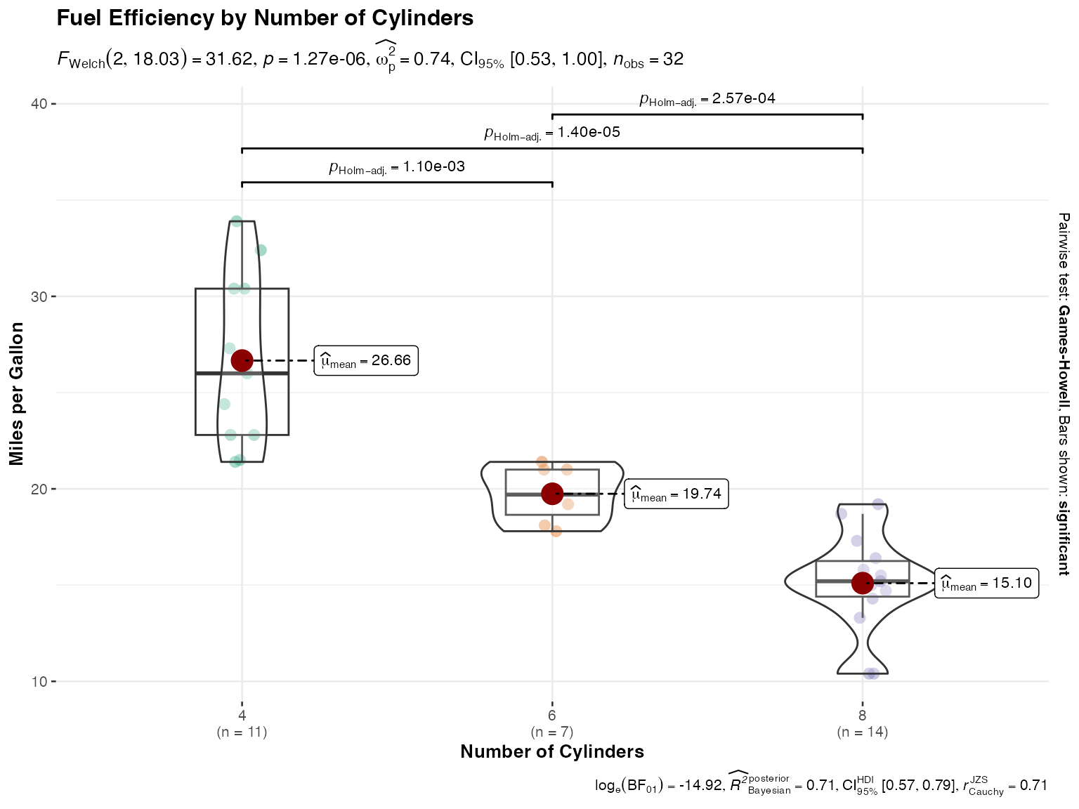
The jjbetweenstats() function creates box-violin plots to compare continuous variables between independent groups. It automatically performs appropriate statistical tests (parametric, non-parametric, robust, or Bayesian) and displays the results.

# Underlying function that jjbetweenstats() wraps
ggstatsplot::ggbetweenstats(
  data = mtcars,
  x = cyl,
  y = mpg,
  type = "parametric",
  pairwise.comparisons = TRUE,
  pairwise.display = "significant",
  centrality.plotting = TRUE,
  title = "Fuel Efficiency by Number of Cylinders",
  xlab = "Number of Cylinders",
  ylab = "Miles per Gallon"
)

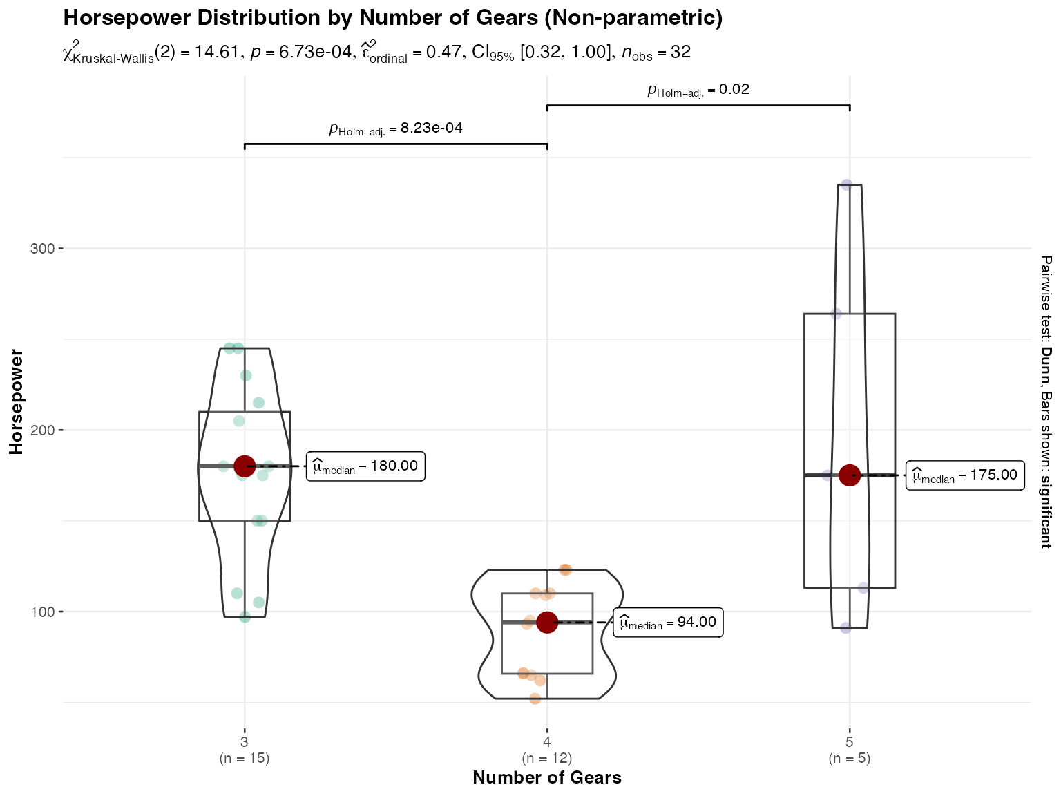
Customizing the analysis type

You can choose different types of statistical analyses:

# Non-parametric analysis with Kruskal-Wallis test
ggstatsplot::ggbetweenstats(
  data = mtcars,
  x = gear,
  y = hp,
  type = "nonparametric",
  centrality.plotting = TRUE,
  centrality.type = "nonparametric",
  title = "Horsepower Distribution by Number of Gears (Non-parametric)",
  xlab = "Number of Gears",
  ylab = "Horsepower"
)

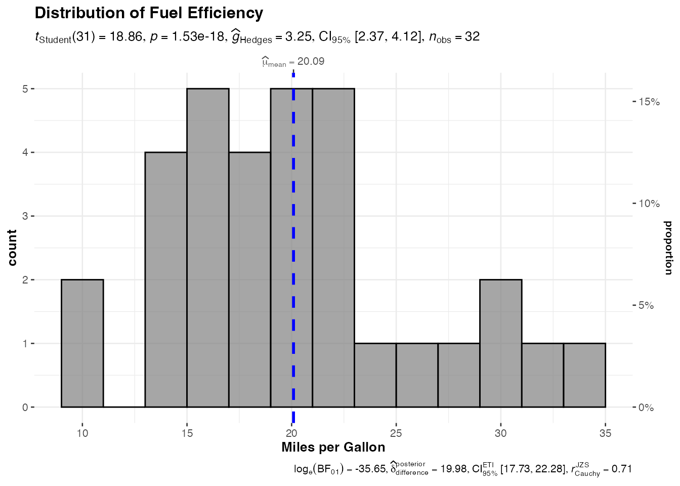
Histograms with `jjhistostats()`

The jjhistostats() function creates histograms with overlaid density curves and statistical test results against a specified test value.

# Underlying function that jjhistostats() wraps
ggstatsplot::gghistostats(
  data = mtcars,
  x = mpg,
  type = "parametric",
  normal.curve = TRUE,
  binwidth = 2,
  title = "Distribution of Fuel Efficiency",
  xlab = "Miles per Gallon"
)

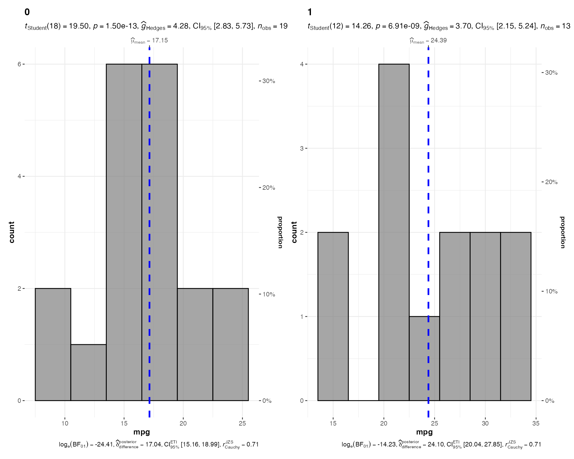
Grouped histograms

You can also create histograms split by a grouping variable:

# Grouped histogram
ggstatsplot::grouped_gghistostats(
  data = mtcars,
  x = mpg,
  grouping.var = am,
  binwidth = 3,
  title.prefix = "Transmission Type",
  normal.curve = TRUE
)

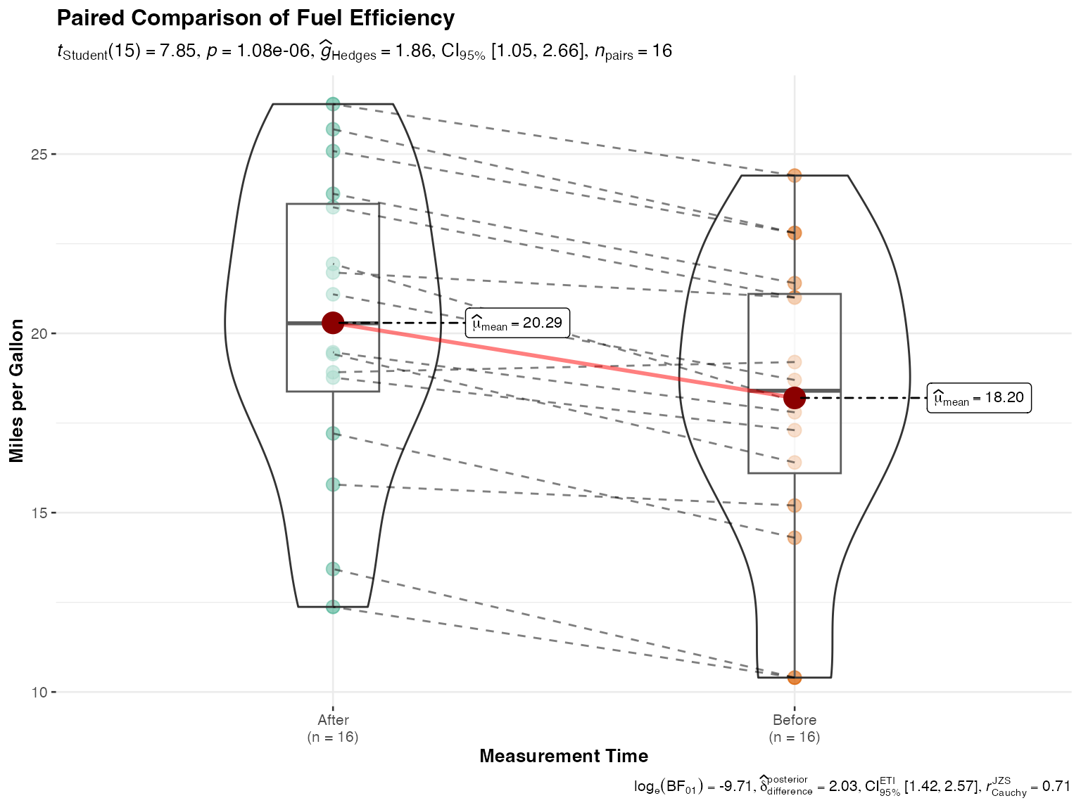
Within-group comparisons with `jjwithinstats()`

The jjwithinstats() function is designed for repeated measures or paired comparisons. It shows individual trajectories and performs appropriate paired tests.

# Create paired data for demonstration
library(tidyr)
library(dplyr)
#> 
#> Attaching package: 'dplyr'
#> The following objects are masked from 'package:stats':
#> 
#>     filter, lag
#> The following objects are masked from 'package:base':
#> 
#>     intersect, setdiff, setequal, union

# Simulate paired measurements (e.g., before and after treatment)
paired_data <- data.frame(
  id = rep(1:16, 2),
  condition = rep(c("Before", "After"), each = 16),
  value = c(mtcars$mpg[1:16], mtcars$mpg[1:16] + rnorm(16, mean = 2, sd = 1))
)

# Underlying function that jjwithinstats() wraps
ggstatsplot::ggwithinstats(
  data = paired_data,
  x = condition,
  y = value,
  paired = TRUE,
  id = id,
  type = "parametric",
  pairwise.comparisons = TRUE,
  title = "Paired Comparison of Fuel Efficiency",
  xlab = "Measurement Time",
  ylab = "Miles per Gallon"
)

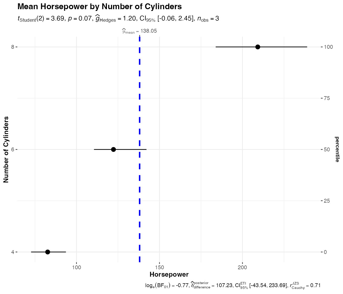
Dot plots with `jjdotplotstats()`

The jjdotplotstats() function creates Cleveland dot plots showing group means or medians with confidence intervals. This is particularly useful for comparing multiple groups when you want to emphasize the central tendency and uncertainty.

# Underlying function that jjdotplotstats() wraps
ggstatsplot::ggdotplotstats(
  data = mtcars,
  x = hp,
  y = cyl,
  type = "parametric",
  centrality.plotting = TRUE,
  title = "Mean Horsepower by Number of Cylinders",
  xlab = "Horsepower",
  ylab = "Number of Cylinders"
)

Statistical details

All these functions provide:

Automatic statistical testing: Based on the type parameter, appropriate tests are selected:
- Parametric: t-test, ANOVA, paired t-test
- Non-parametric: Mann-Whitney U, Kruskal-Wallis, Wilcoxon signed-rank
- Robust: Yuen’s trimmed means test, heteroscedastic ANOVA
- Bayesian: Bayes Factor analysis
Effect sizes: Appropriate effect size measures are computed and displayed:
- Cohen’s d, Hedge’s g (for t-tests)
- Eta-squared, omega-squared (for ANOVA)
- r (for non-parametric tests)
Pairwise comparisons: When comparing multiple groups, post-hoc pairwise comparisons are available with p-value adjustment methods.

Usage in jamovi

These functions are integrated into the jamovi interface where they provide:

Point-and-click variable selection
Interactive options for customizing plots
Automatic handling of missing data
Export options for plots and results

To use these in jamovi:

Install the jjstatsplot module from the jamovi library
Load your dataset
Navigate to JJStatsPlot → Continuous menu
Select the appropriate analysis
Configure options through the user-friendly interface

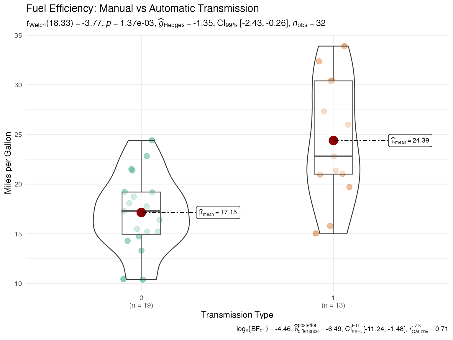
Advanced customization

While the jamovi interface provides the most common options, R users can access additional customization through the underlying ggstatsplot functions:

# Example with extensive customization
ggstatsplot::ggbetweenstats(
  data = mtcars,
  x = am,
  y = mpg,
  type = "parametric",
  # Visual customization
  violin.args = list(width = 0.5, alpha = 0.2),
  boxplot.args = list(width = 0.2, alpha = 0.5),
  point.args = list(alpha = 0.5, size = 3, position = ggplot2::position_jitter(width = 0.1)),
  # Statistical options
  conf.level = 0.99,
  effsize.type = "unbiased",
  # Theming
  ggtheme = ggplot2::theme_minimal(),
  # Labels
  title = "Fuel Efficiency: Manual vs Automatic Transmission",
  subtitle = "99% confidence intervals shown",
  xlab = "Transmission Type",
  ylab = "Miles per Gallon",
  caption = "Data: Motor Trend Car Road Tests"
)

Summary

The continuous comparison functions in jjstatsplot provide:

Comprehensive statistical analyses with minimal code
Publication-ready visualizations
Automatic selection of appropriate statistical tests
Integration with jamovi’s graphical interface
Flexibility for advanced R users

These tools make it easy to perform rigorous statistical comparisons while creating informative visualizations suitable for both exploration and presentation.

Between-group comparisons with jjbetweenstats()