R Programming Guide for jjstatsplot
ClinicoPath Development Team
2025-06-30
Source:vignettes/general-14-r-programming-guide.Rmd
general-14-r-programming-guide.RmdUsing jjstatsplot Functions in R
This guide demonstrates how to use jjstatsplot functions directly in R for programmatic statistical visualization. While these functions are designed for jamovi integration, they can be powerful tools in R workflows.
Installation and Setup
# Install from GitHub
if (!require(devtools)) install.packages("devtools")
devtools::install_github("sbalci/jjstatsplot")

# Install dependencies if needed
install.packages(c("ggplot2", "ggstatsplot", "dplyr", "jmvcore"))
library(ClinicoPath)
#> Registered S3 method overwritten by 'future':
#>   method               from
#>   all.equal.connection parallelly
#> Warning: replacing previous import 'dplyr::select' by 'jmvcore::select' when
#> loading 'ClinicoPath'
#> Warning: replacing previous import 'cutpointr::roc' by 'pROC::roc' when loading
#> 'ClinicoPath'
#> Warning: replacing previous import 'cutpointr::auc' by 'pROC::auc' when loading
#> 'ClinicoPath'
#> Warning: replacing previous import 'magrittr::extract' by 'tidyr::extract' when
#> loading 'ClinicoPath'
#> Warning in check_dep_version(): ABI version mismatch:
#> lme4 was built with Matrix ABI version 1
#> Current Matrix ABI version is 0
#> Please re-install lme4 from source or restore original 'Matrix' package
#> Warning: replacing previous import 'jmvcore::select' by 'dplyr::select' when
#> loading 'ClinicoPath'
#> Registered S3 methods overwritten by 'ggpp':
#>   method                  from
#>   heightDetails.titleGrob ggplot2
#>   widthDetails.titleGrob  ggplot2
#> Warning: replacing previous import 'DataExplorer::plot_histogram' by
#> 'grafify::plot_histogram' when loading 'ClinicoPath'
#> Warning: replacing previous import 'ROCR::plot' by 'graphics::plot' when
#> loading 'ClinicoPath'
#> Warning: replacing previous import 'dplyr::select' by 'jmvcore::select' when
#> loading 'ClinicoPath'
#> Warning: replacing previous import 'tibble::view' by 'summarytools::view' when
#> loading 'ClinicoPath'
library(ggplot2)
#> Warning: package 'ggplot2' was built under R version 4.3.3
library(dplyr)
#>
#> Attaching package: 'dplyr'
#> The following objects are masked from 'package:stats':
#>
#>     filter, lag
#> The following objects are masked from 'package:base':
#>
#>     intersect, setdiff, setequal, union

# Load example data
data(mtcars)
data(iris)
Understanding jjstatsplot Function Structure
Return Objects
All jjstatsplot functions return jamovi results objects with: -
$plot - The main ggplot2 object - $plot2 -
Secondary plot (when grouping variables are used) - Statistical results
and metadata
Basic Pattern
# General function signature
result <- jj[function_name](
  data = your_data,
  dep = dependent_variable(s),
  group = grouping_variable,
  grvar = grouping_for_separate_plots,
  # Additional options...
)

# Extract the plot
plot <- result$plot
print(plot)
Function-by-Function Guide
1. Histogram Analysis - jjhistostats()
# Basic histogram
hist_result <- jjhistostats(
  data = mtcars,
  dep = "mpg",
  grvar = NULL
)

# Extract and display plot
hist_result$plot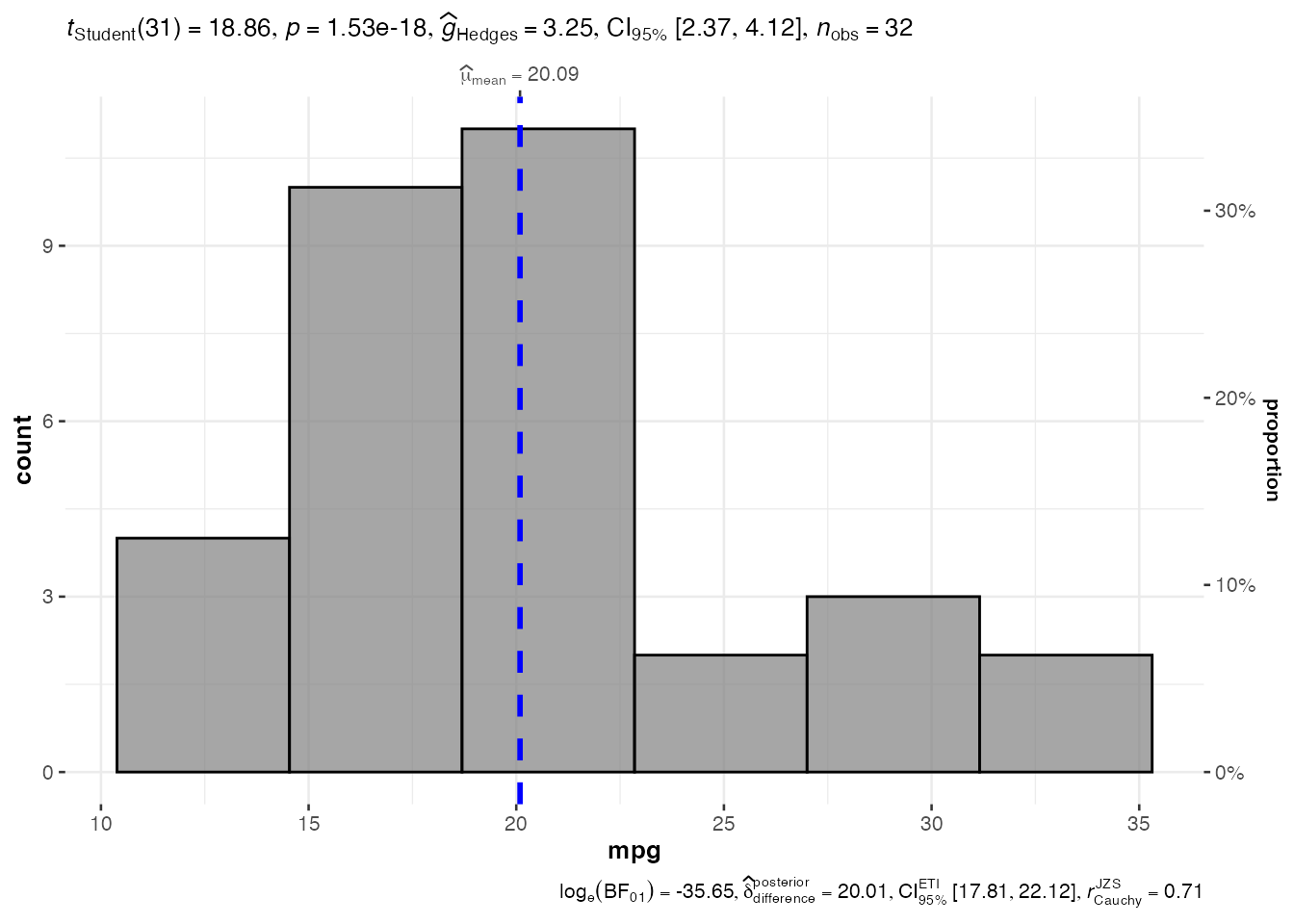
# Histogram with grouping
hist_grouped <- jjhistostats(
  data = mtcars,
  dep = "mpg",
  grvar = "cyl"
)

# Multiple plots created
hist_grouped$plot2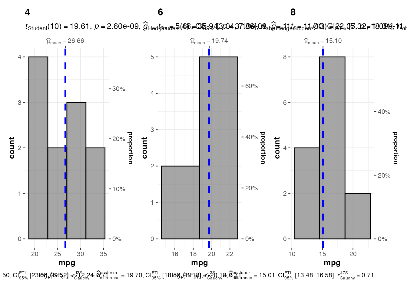
2. Scatter Plots - jjscatterstats()
# Basic scatter plot
scatter_result <- jjscatterstats(
  data = mtcars,
  dep = "mpg",
  group = "hp",
  grvar = NULL
)

scatter_result$plot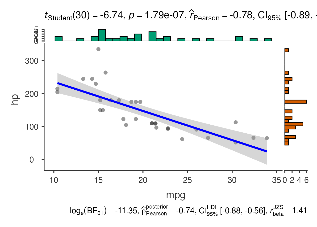
# Scatter plot with grouping variable
scatter_grouped <- jjscatterstats(
  data = mtcars,
  dep = "mpg",
  group = "hp",
  grvar = "cyl"
)

scatter_grouped$plot2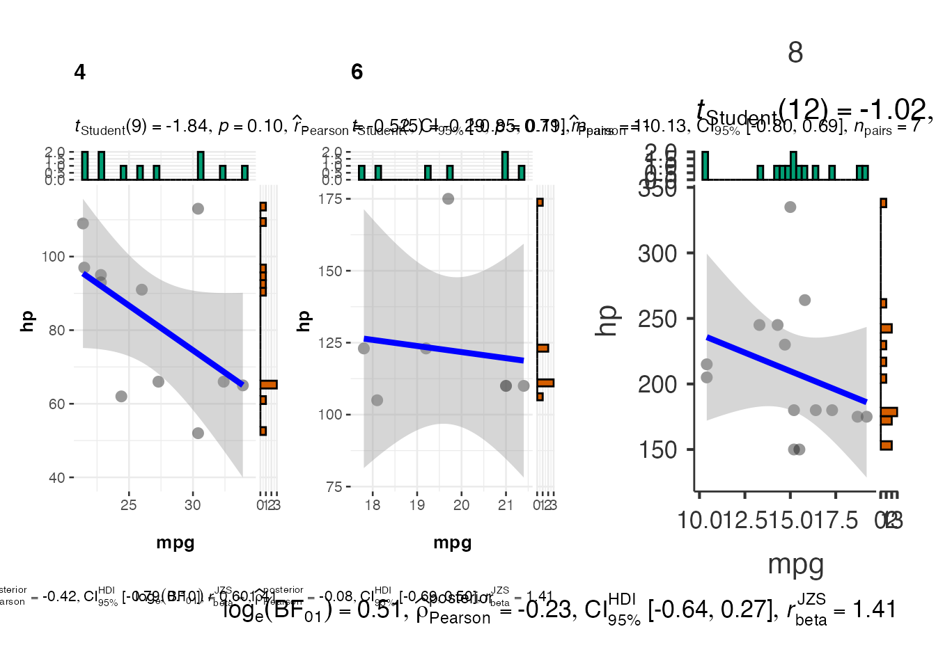
3. Box-Violin Plots - jjbetweenstats()
# Between-groups comparison
between_result <- jjbetweenstats(
  data = iris,
  dep = "Sepal.Length",
  group = "Species"
)

between_result$plot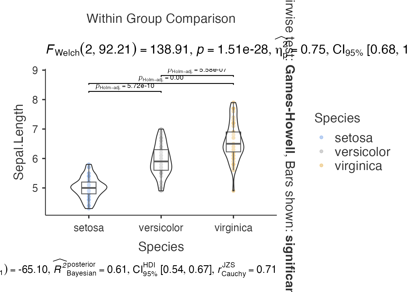
# Multiple dependent variables
between_multi <- jjbetweenstats(
  data = iris,
  dep = c("Sepal.Length", "Petal.Length"),
  group = "Species"
)

between_multi$plot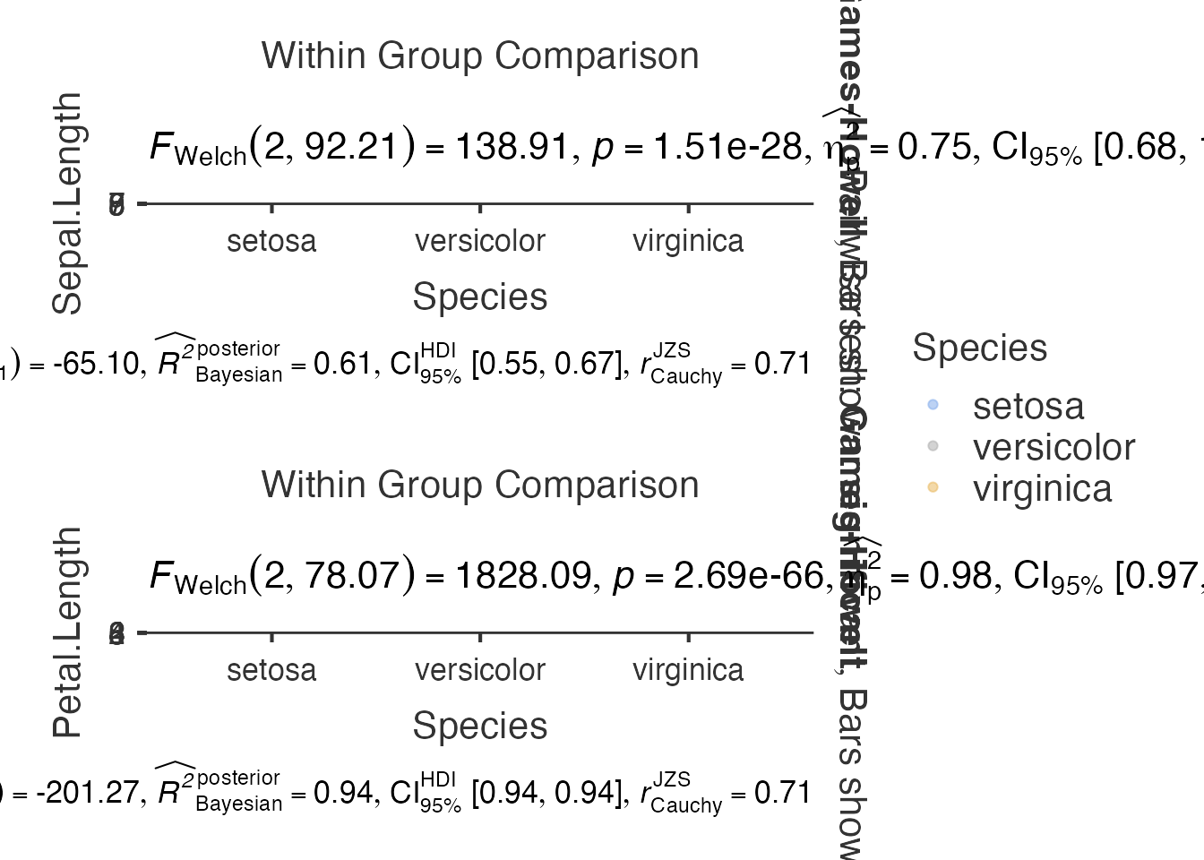
4. Correlation Matrix - jjcorrmat()
# Correlation matrix
corr_result <- jjcorrmat(
  data = mtcars,
  dep = c("mpg", "hp", "wt", "qsec"),
  grvar = NULL
)

corr_result$plot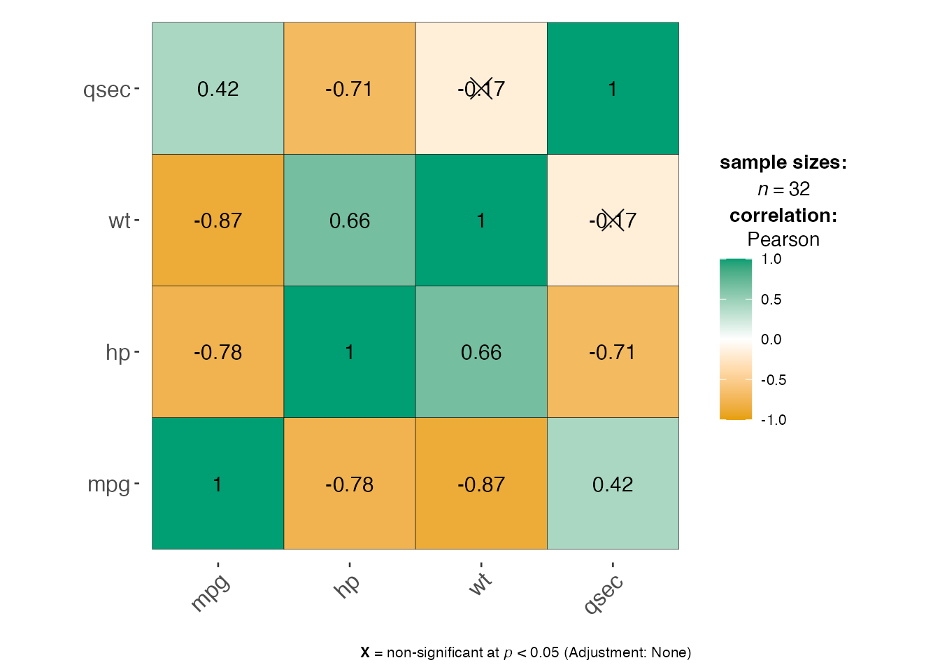
5. Dot Plots - jjdotplotstats()
# Dot plot for group comparisons
dot_result <- jjdotplotstats(
  data = mtcars,
  dep = "mpg",
  group = "cyl",
  grvar = NULL
)

dot_result$plot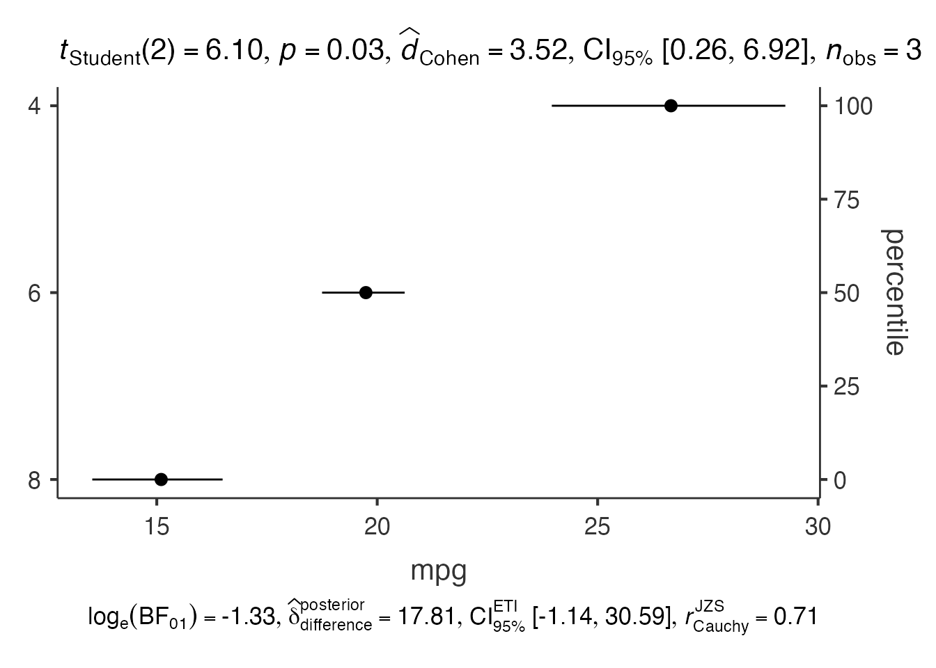
6. Bar Charts - jjbarstats()
# Bar chart for categorical data
bar_result <- jjbarstats(
  data = mtcars,
  dep = "cyl",
  group = "am",
  grvar = NULL
)

bar_result$plot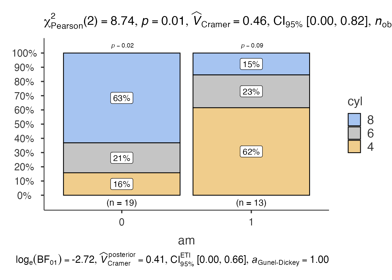
7. Pie Charts - jjpiestats()
# Pie chart
pie_result <- jjpiestats(
  data = mtcars,
  dep = "cyl",
  group = NULL,
  grvar = NULL
)

pie_result$plot1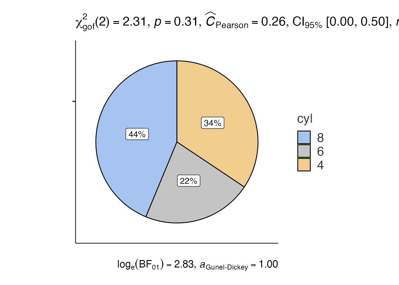
8. Within-Subjects Analysis - jjwithinstats()
# For repeated measures data
# Note: This requires appropriate data structure
# Creating example with iris data (not true repeated measures)
within_result <- jjwithinstats(
  data = iris,
  dep1 = "Sepal.Length",
  dep2 = "Sepal.Width",
  dep3 = NULL,
  dep4 = NULL
)

within_result$plot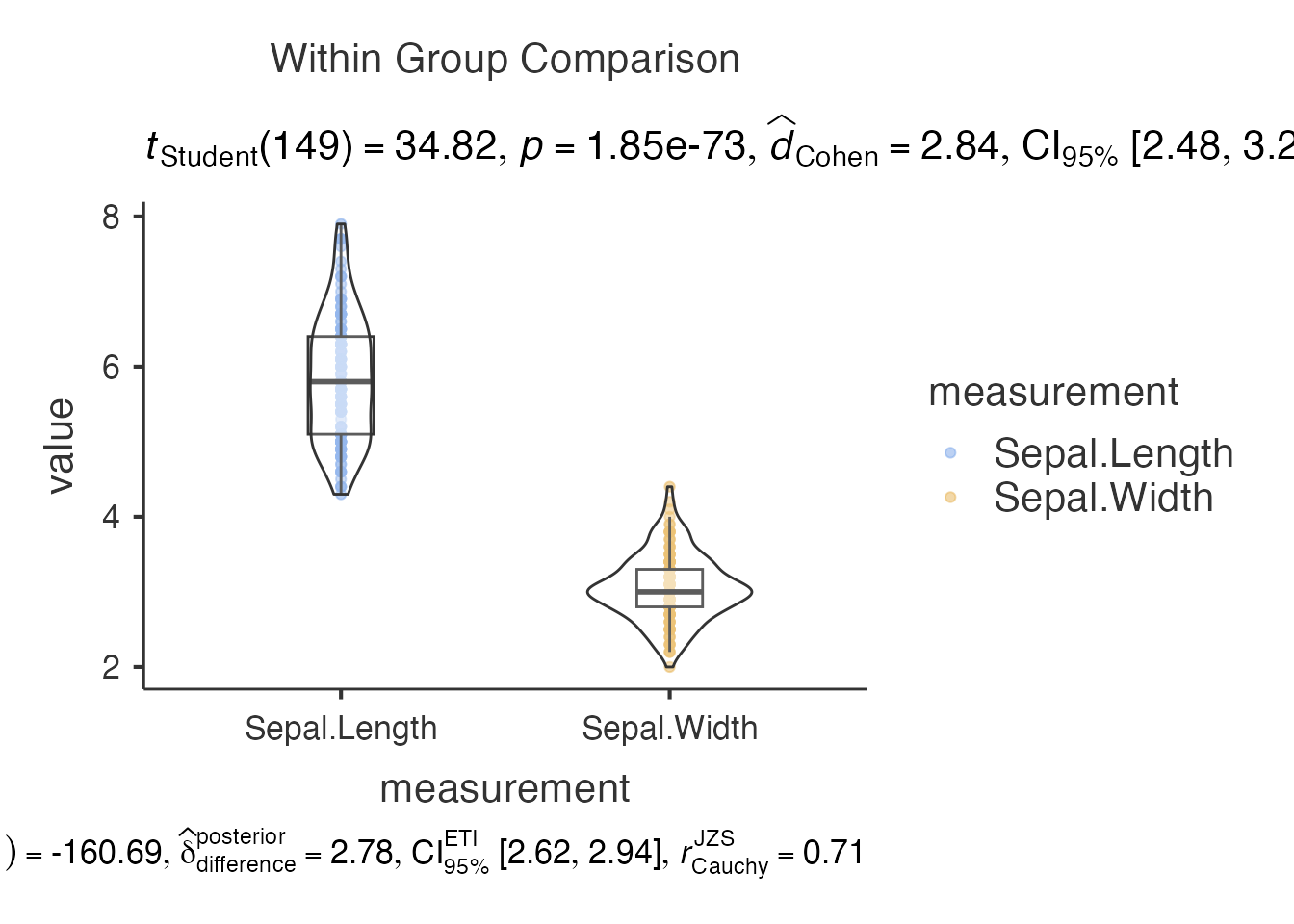
Advanced Usage Patterns
Working with Multiple Variables
# Analyze multiple dependent variables simultaneously
multi_hist <- jjhistostats(
  data = iris,
  dep = c("Sepal.Length", "Sepal.Width", "Petal.Length"),
  grvar = NULL
)

# This creates a combined plot
multi_hist$plot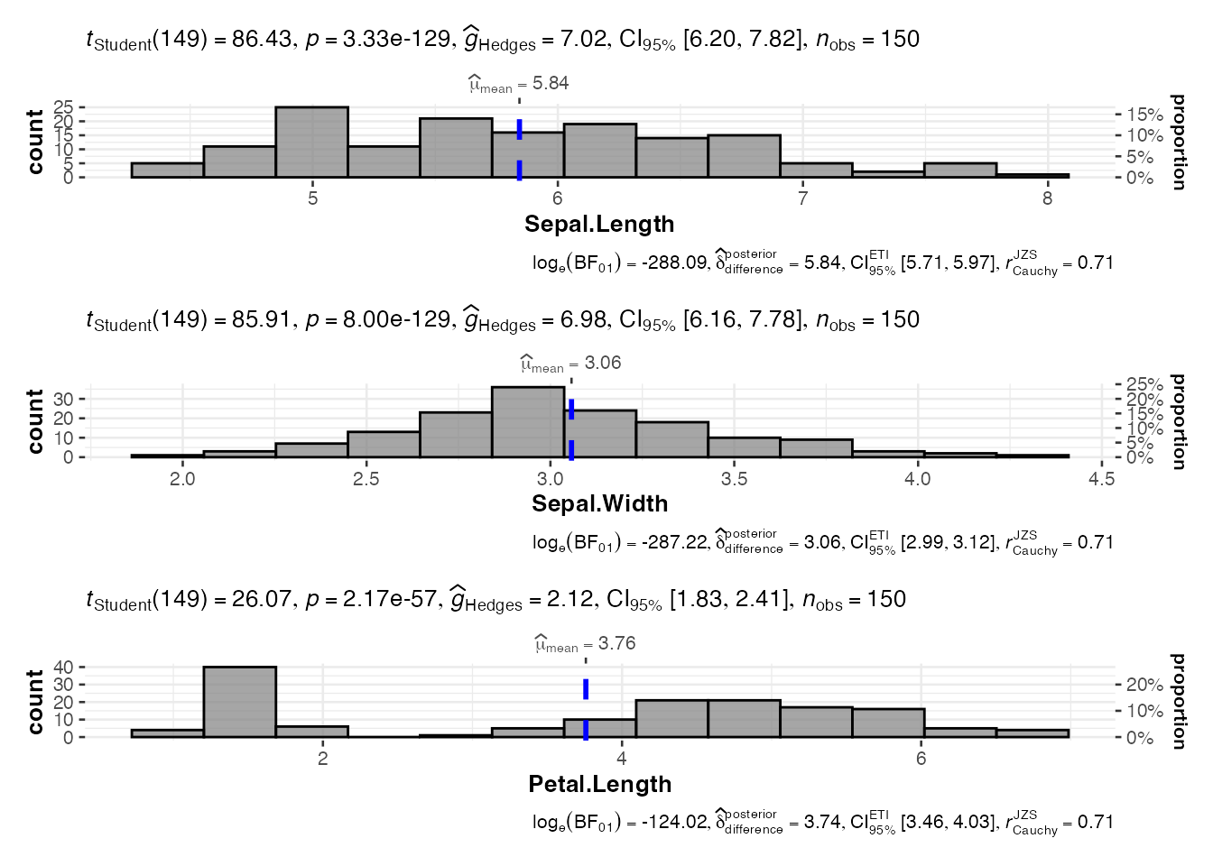
Combining with dplyr Workflows
# Preprocessing with dplyr, then plotting
mtcars_processed <- mtcars %>%
  mutate(
    cyl_factor = factor(cyl, labels = c("4-cyl", "6-cyl", "8-cyl")),
    am_factor = factor(am, labels = c("Automatic", "Manual"))
  ) %>%
  filter(hp > 100)

# Use processed data
result <- jjbetweenstats(
  data = mtcars_processed,
  dep = "mpg",
  group = "cyl_factor"
)

result$plot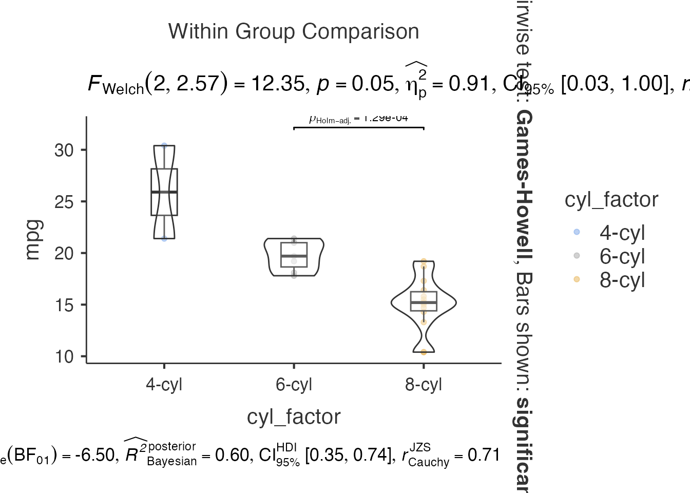
Extracting Statistical Information
# jjstatsplot functions return rich statistical information
corr_analysis <- jjcorrmat(
  data = mtcars[, c("mpg", "hp", "wt")],
  dep = c("mpg", "hp", "wt"),
  grvar = NULL
)

# The plot contains statistical annotations
print(corr_analysis$plot)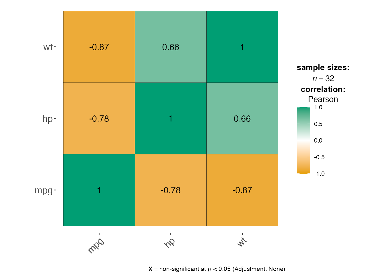
# Access underlying data if needed (structure varies by function)
str(corr_analysis, max.level = 2)
#> Classes 'jjcorrmatResults', 'Group', 'ResultsElement', 'R6' <jjcorrmatResults>
#>   Inherits from: <Group>
#>   Public:
#>     .createImages: function (...)
#>     .has: function (name)
#>     .lookup: function (path)
#>     .render: function (...)
#>     .setKey: function (key, index)
#>     .setName: function (name)
#>     .setParent: function (parent)
#>     .update: function ()
#>     add: function (item)
#>     analysis: active binding
#>     asDF: active binding
#>     asProtoBuf: function (incAsText = FALSE, status = NULL, prepend = NULL, append = NULL,
#>     asString: function ()
#>     clear: function ()
#>     clone: function (deep = FALSE)
#>     fromProtoBuf: function (pb, oChanges, vChanges)
#>     get: function (name)
#>     getBoundVars: function (expr)
#>     getRefs: function (recurse = FALSE)
#>     index: active binding
#>     initialize: function (options)
#>     insert: function (index, item)
#>     isFilled: function ()
#>     isNotFilled: function ()
#>     itemNames: active binding
#>     items: active binding
#>     key: active binding
#>     name: active binding
#>     options: active binding
#>     parent: active binding
#>     path: active binding
#>     plot: active binding
#>     plot2: active binding
#>     print: function ()
#>     remove: function (name)
#>     requiresData: active binding
#>     resetVisible: function ()
#>     root: active binding
#>     saveAs: function (file, format)
#>     setError: function (message)
#>     setRefs: function (refs)
#>     setState: function (state)
#>     setStatus: function (status)
#>     setTitle: function (title)
#>     setVisible: function (visible = TRUE)
#>     state: active binding
#>     status: active binding
#>     title: active binding
#>     todo: active binding
#>     visible: active binding
#>   Private:
#>     .clearWith: list
#>     .error: NA
#>     .index: NA
#>     .items: list
#>     .key: NA
#>     .name:
#>     .options: jjcorrmatOptions, Options, R6
#>     .parent: jjcorrmatClass, jjcorrmatBase, Analysis, R6
#>     .refs: ggplot2 ggstatsplot ClinicoPathJamoviModule
#>     .stale: TRUE
#>     .state: NULL
#>     .status: none
#>     .titleExpr: Correlation Matrix
#>     .titleValue: Correlation Matrix
#>     .updated: TRUE
#>     .visibleExpr: NULL
#>     .visibleValue: TRUE
#>     deep_clone: function (name, value)
Customization and Theming
Plot Modifications
# Extract base plot and modify
base_plot <- jjscatterstats(
  data = mtcars,
  dep = "mpg",
  group = "hp",
  grvar = NULL
)$plot

# Add custom modifications
tryCatch({
  custom_plot <- base_plot +
    labs(
      title = "Fuel Efficiency vs Horsepower",
      subtitle = "Modified jjstatsplot output",
      caption = "Data: mtcars dataset"
    ) +
    theme_minimal() +
    theme(
      plot.title = element_text(size = 16, face = "bold"),
      plot.subtitle = element_text(size = 12)
    )

  print(custom_plot)
}, error = function(e) {
  cat("Plot customization temporarily unavailable due to compatibility issues.\n")
  print(base_plot)
})
#> Plot customization temporarily unavailable due to compatibility issues.
Integration with R Markdown
Chunk Options for Optimal Display
# Recommended chunk options for jjstatsplot in R Markdown:

# ```{r plot-name, fig.width=8, fig.height=6, dpi=300}
# result <- jjhistostats(data = mydata, dep = "variable")
# result$plot
# ```
Creating Function Wrappers
# Create convenience wrappers for common analyses
quick_histogram <- function(data, variable, group_by = NULL) {
  result <- jjhistostats(
    data = data,
    dep = variable,
    grvar = group_by
  )

  if (is.null(group_by)) {
    return(result$plot)
  } else {
    return(result$plot2)
  }
}

# Usage
tryCatch({
  quick_histogram(mtcars, "mpg", "cyl")
}, error = function(e) {
  cat("Function wrapper example temporarily unavailable due to data compatibility issues.\n")
  cat("Error:", e$message, "\n")
})
#> Function wrapper example temporarily unavailable due to data compatibility issues.
#> Error: 'names' attribute [11] must be the same length as the vector [0]
Batch Analysis Functions
# Function to create multiple plots
analyze_variables <- function(data, variables, group_var = NULL) {
  plots <- list()

  for (var in variables) {
    result <- jjhistostats(
      data = data,
      dep = var,
      grvar = group_var
    )

    plots[[var]] <- if (is.null(group_var)) result$plot else result$plot2
  }

  return(plots)
}

# Create multiple histograms
numeric_vars <- c("mpg", "hp", "wt")
tryCatch({
  plot_list <- analyze_variables(mtcars, numeric_vars, "cyl")
  # Display first plot
  print(plot_list$mpg)
}, error = function(e) {
  cat("Batch analysis example temporarily unavailable due to data compatibility issues.\n")
  cat("Error:", e$message, "\n")
})
#> Batch analysis example temporarily unavailable due to data compatibility issues.
#> Error: 'names' attribute [11] must be the same length as the vector [0]
Error Handling and Debugging
Common Issues and Solutions
# Safe function wrapper with error handling
safe_jjhistostats <- function(data, dep, ...) {
  tryCatch({
    result <- jjhistostats(data = data, dep = dep, ...)
    return(result$plot)
  }, error = function(e) {
    message("Error creating histogram: ", e$message)
    return(NULL)
  })
}

# Usage with potential problematic data
plot_result <- safe_jjhistostats(mtcars, "nonexistent_variable")
Data Validation
# Function to check data before analysis
validate_data <- function(data, variables) {
  issues <- list()

  # Check if variables exist
  missing_vars <- variables[!variables %in% names(data)]
  if (length(missing_vars) > 0) {
    issues$missing_variables <- missing_vars
  }

  # Check for sufficient data
  for (var in variables) {
    if (var %in% names(data)) {
      non_missing <- sum(!is.na(data[[var]]))
      if (non_missing < 10) {
        issues$insufficient_data <- c(issues$insufficient_data, var)
      }
    }
  }

  return(issues)
}

# Example usage
issues <- validate_data(mtcars, c("mpg", "hp", "nonexistent"))
print(issues)
#> $missing_variables
#> [1] "nonexistent"
Performance Considerations
Large Datasets
# For large datasets, consider sampling
large_data_plot <- function(data, dep, sample_size = 1000) {
  if (nrow(data) > sample_size) {
    sampled_data <- data[sample(nrow(data), sample_size), ]
    message("Sampling ", sample_size, " rows from ", nrow(data), " total rows")
    data <- sampled_data
  }

  jjhistostats(data = data, dep = dep, grvar = NULL)$plot
}
Best Practices Summary
1. Function Usage
- Always check return structure:
$plotvs$plot2 - Handle missing data appropriately
- Validate variable names before analysis
2. Data Preparation
- Use meaningful variable names and factor labels
- Ensure appropriate data types (numeric, factor)
- Consider data transformations when needed
3. Workflow Integration
- Combine with dplyr for data preprocessing
- Create wrapper functions for repeated analyses
- Use error handling for robust scripts
4. Output Management
- Extract plots with
result$plot - Modify plots using standard ggplot2 syntax
- Save plots with appropriate dimensions and resolution
5. Documentation
- Document your analysis choices
- Include variable descriptions
- Report statistical assumptions and violations
This guide provides a foundation for using jjstatsplot functions programmatically in R. The functions offer a convenient way to create publication-ready statistical visualizations with minimal code while maintaining access to the underlying ggplot2 objects for further customization.