Comprehensive Bar Chart Analysis with jjbarstats
ClinicoPath Development Team
2025-07-13
Source:vignettes/jjstatsplot-23-jjbarstats-comprehensive.Rmd
jjstatsplot-23-jjbarstats-comprehensive.RmdIntroduction to jjbarstats
The jjbarstats function is a powerful wrapper around the
ggstatsplot package that creates publication-ready bar
charts with automatic statistical testing. This function is designed
specifically for analyzing categorical data relationships in clinical
and research settings.
Key Features
- Automatic Statistical Testing: Performs chi-squared tests, Fisher’s exact tests, or other appropriate tests based on your data
- Multiple Variable Support: Handle single or multiple dependent variables simultaneously
- Grouped Analysis: Split analysis by additional grouping variables
- Flexible Statistical Methods: Choose from parametric, non-parametric, robust, or Bayesian approaches
- Pairwise Comparisons: Automatic post-hoc testing with multiple comparison correction
- Professional Visualization: Publication-ready plots with statistical annotations
When to Use jjbarstats
Use jjbarstats when you need to:
- Compare proportions across different groups
- Analyze treatment effectiveness in clinical trials
- Examine relationships between categorical variables
- Create publication-ready visualizations with statistical tests
- Perform quality improvement analysis
- Analyze survey responses and patient feedback
Basic Usage
Single Dependent Variable Analysis
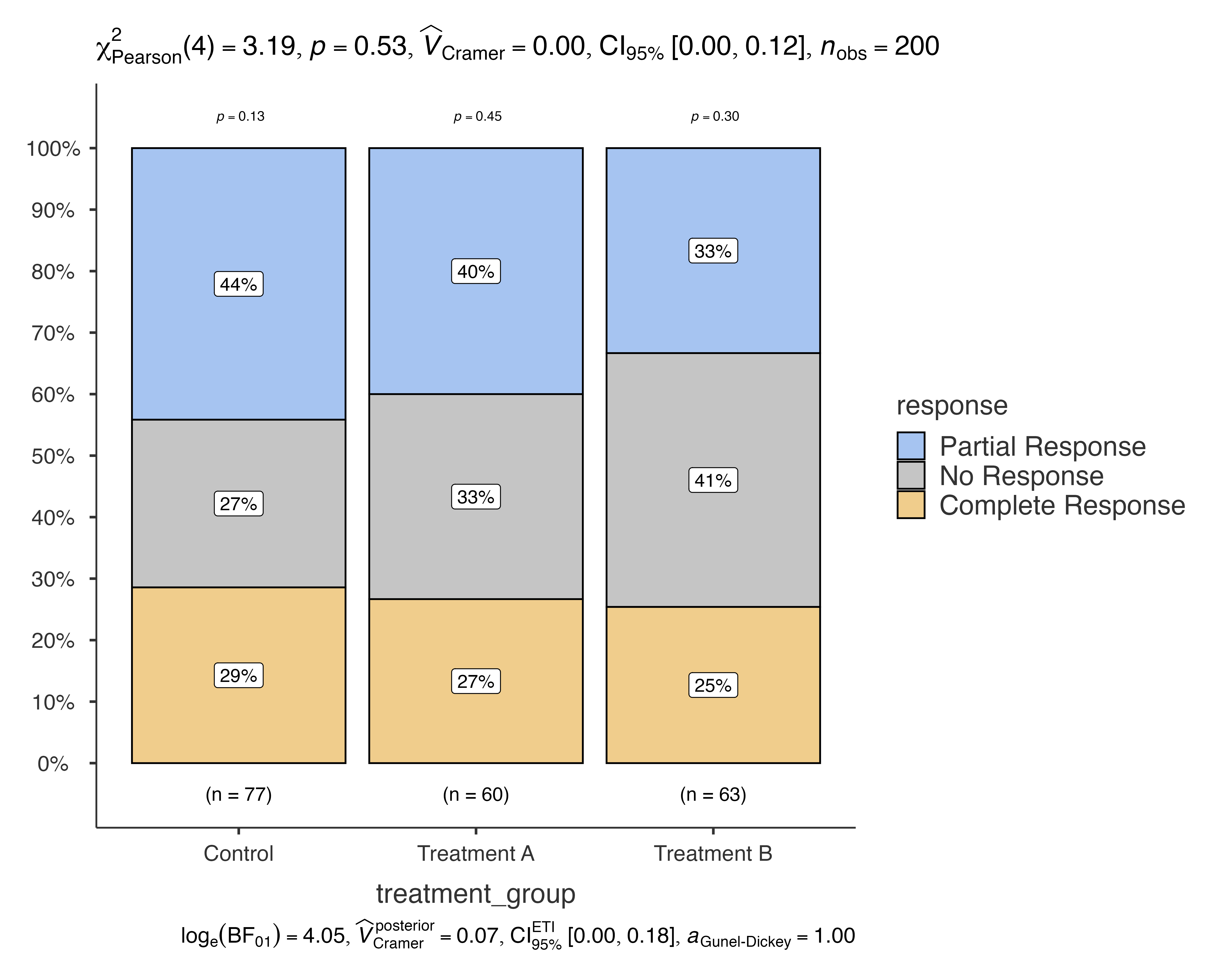
Let’s start with a basic example using medical study data to compare treatment responses across different treatment groups:
# Basic bar chart comparing treatment response across groups
jjbarstats(
  data = medical_study_data,
  dep = response,
  group = treatment_group,
  grvar = NULL
)
#>
#>  BAR CHARTS
#>
#>  Bar chart analysis comparing response by treatment_group.
This creates a bar chart showing the distribution of treatment responses (Complete Response, Partial Response, No Response) across different treatment groups (Control, Treatment A, Treatment B), along with chi-squared test results.
Advanced Statistical Options
Different Statistical Methods
The function supports four different statistical approaches:
Parametric Analysis (Default)
jjbarstats(
  data = patient_satisfaction_data,
  dep = satisfaction_level,
  group = service_type,
  typestatistics = "parametric"
)
#>
#>  BAR CHARTS
#>
#>  Bar chart analysis comparing satisfaction_level by service_type.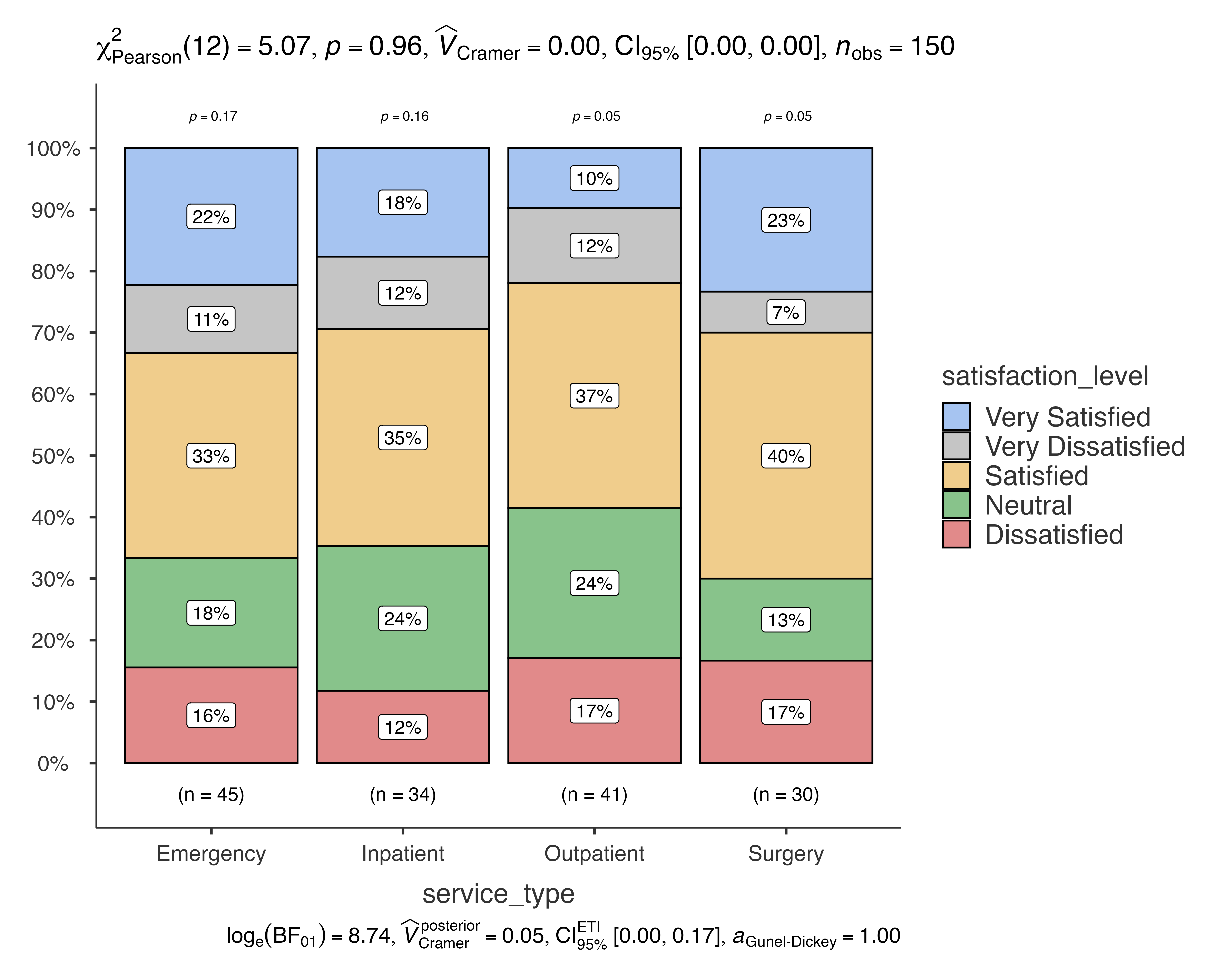
Non-parametric Analysis
jjbarstats(
  data = diagnostic_test_data,
  dep = test_result,
  group = test_method,
  typestatistics = "nonparametric"
)
#>
#>  BAR CHARTS
#>
#>  Bar chart analysis comparing test_result by test_method.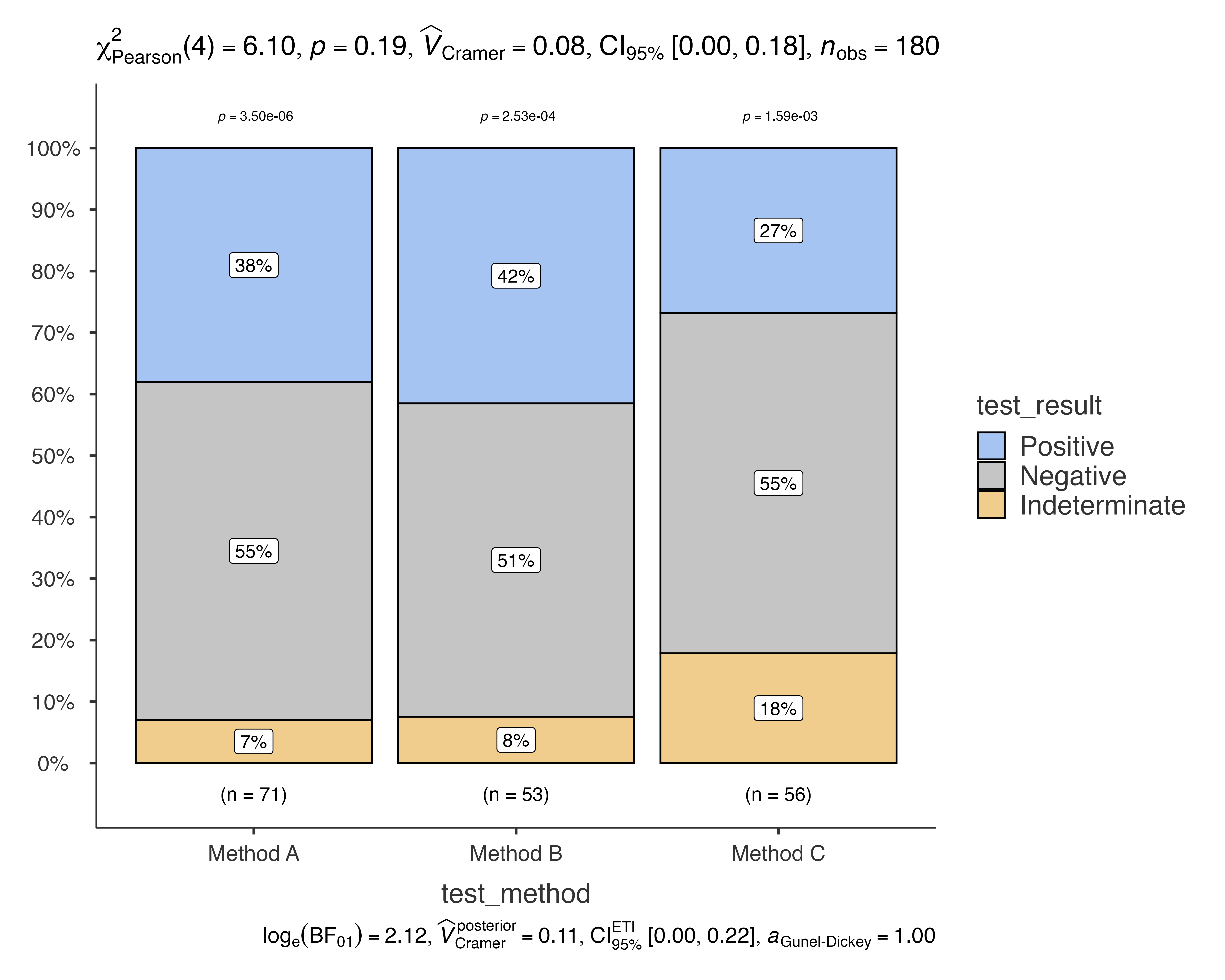
Robust Analysis
jjbarstats(
  data = quality_improvement_data,
  dep = implementation_status,
  group = improvement_category,
  typestatistics = "robust"
)
#>
#>  BAR CHARTS
#>
#>  Bar chart analysis comparing implementation_status by
#>  improvement_category.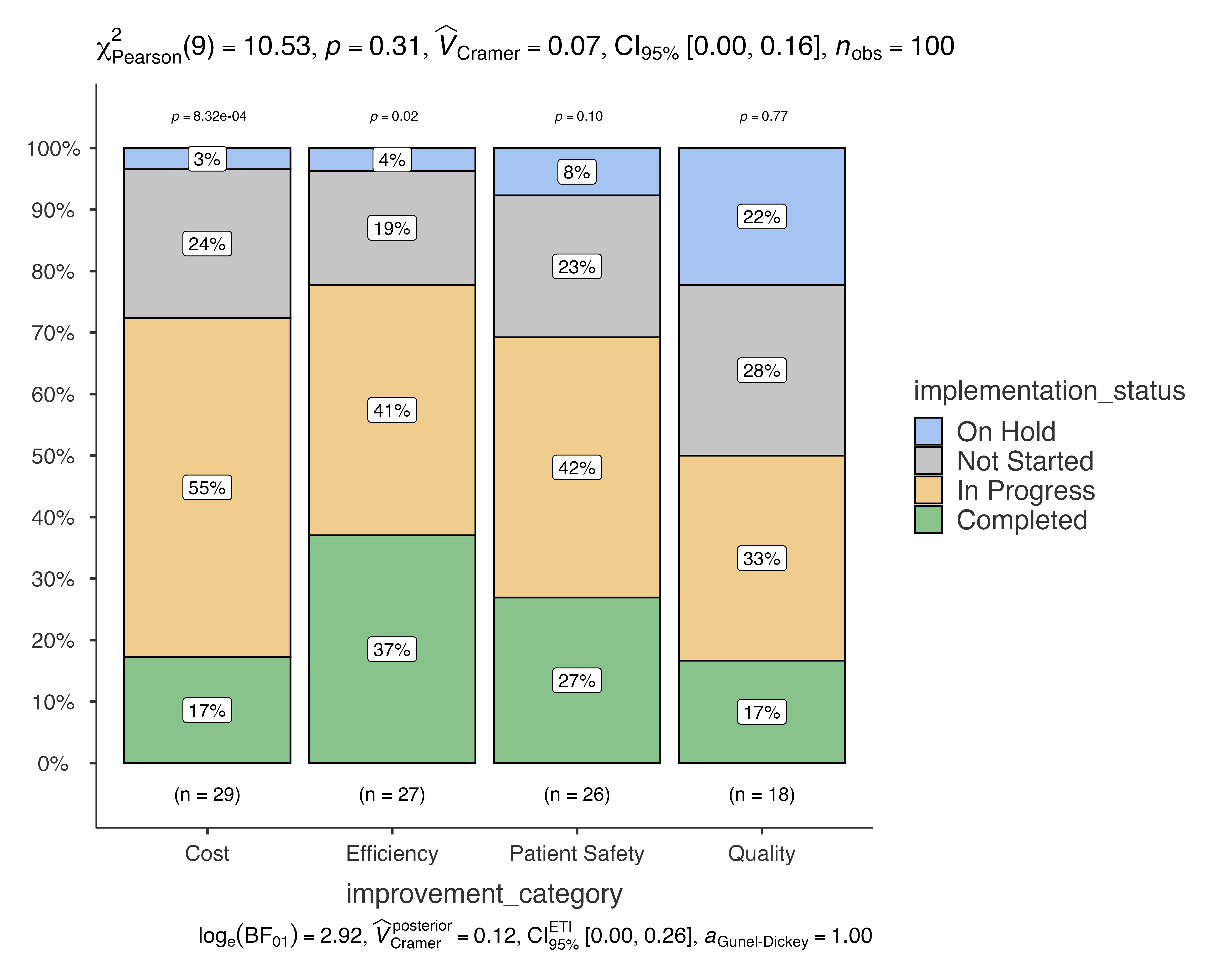
Bayesian Analysis
jjbarstats(
  data = medical_study_data,
  dep = severity,
  group = treatment_group,
  typestatistics = "bayes"
)
#>
#>  BAR CHARTS
#>
#>  Bar chart analysis comparing severity by treatment_group.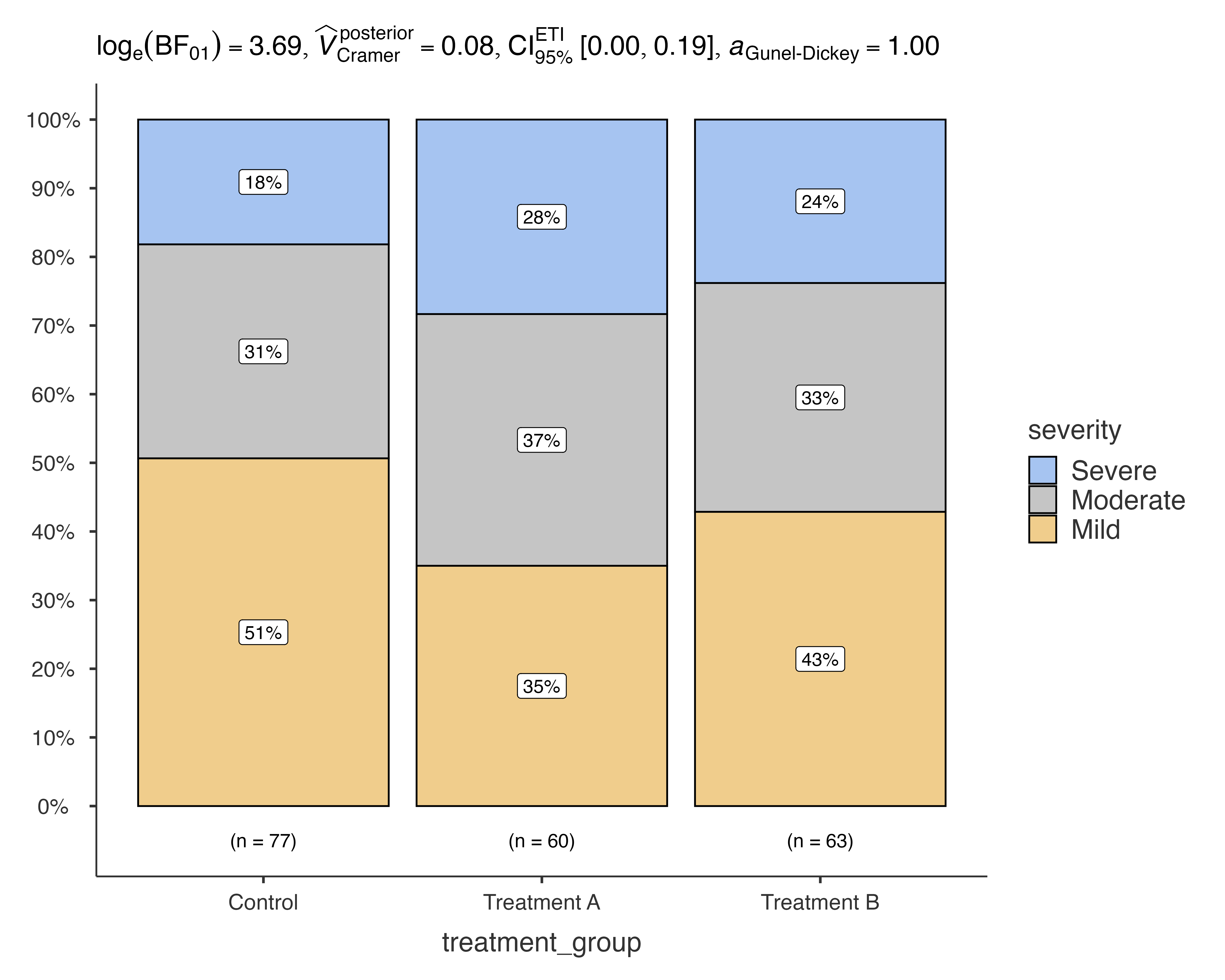
Grouped Analysis with Splitting Variables
Using the grvar Parameter
The grvar parameter allows you to split your analysis by
an additional grouping variable, creating separate plots for each
level:
# Analyze treatment response by treatment group, split by gender
jjbarstats(
  data = medical_study_data,
  dep = response,
  group = treatment_group,
  grvar = gender
)
#>
#>  BAR CHARTS
#>
#>  Bar chart analysis comparing response by treatment_group, grouped by
#>  gender.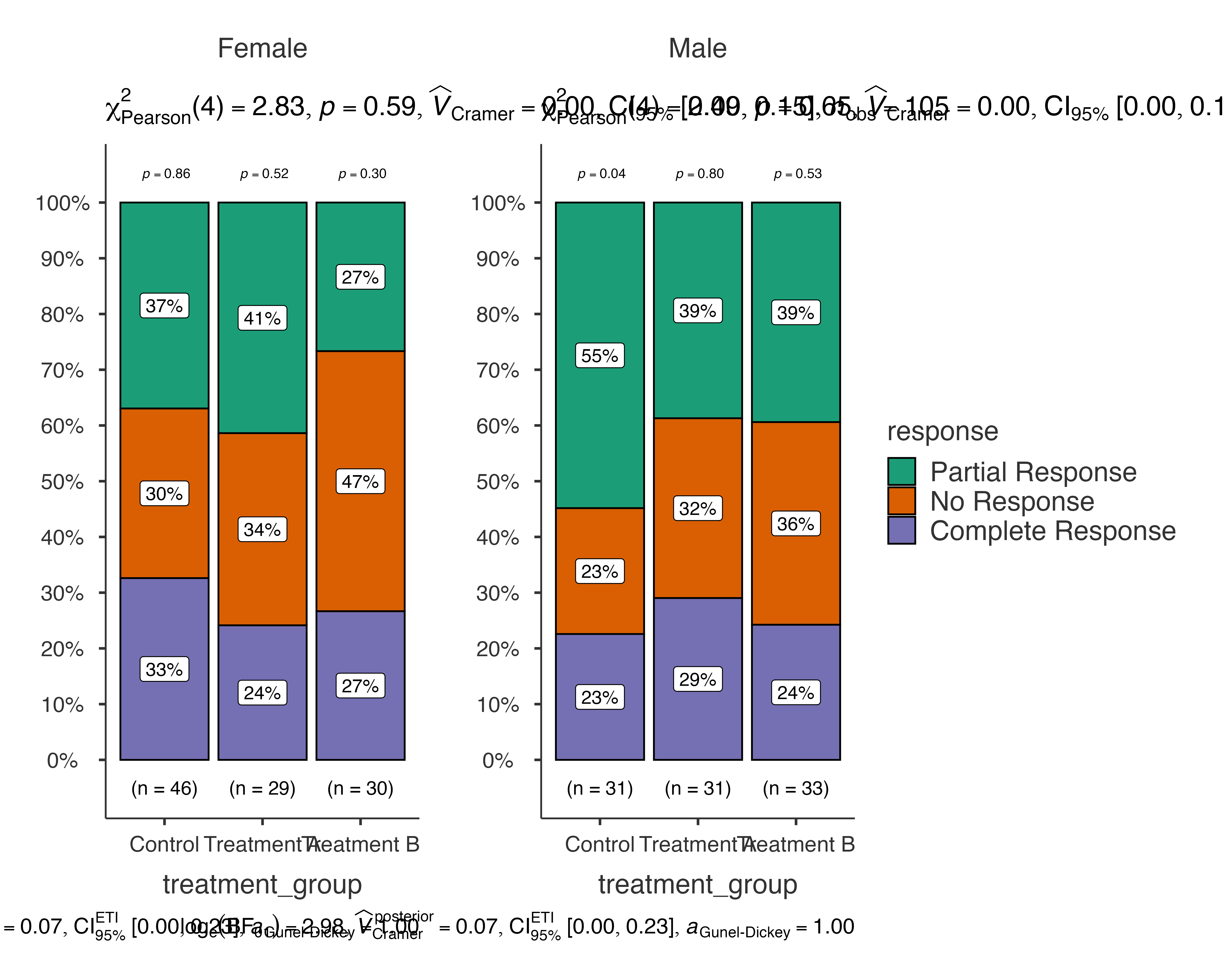
This creates separate bar charts for male and female patients, allowing you to examine whether treatment effects differ by gender.
Complex Grouped Analysis
# Patient satisfaction by service type, split by department
jjbarstats(
  data = patient_satisfaction_data,
  dep = satisfaction_level,
  group = service_type,
  grvar = department
)
#>
#>  BAR CHARTS
#>
#>  Bar chart analysis comparing satisfaction_level by service_type,
#>  grouped by department.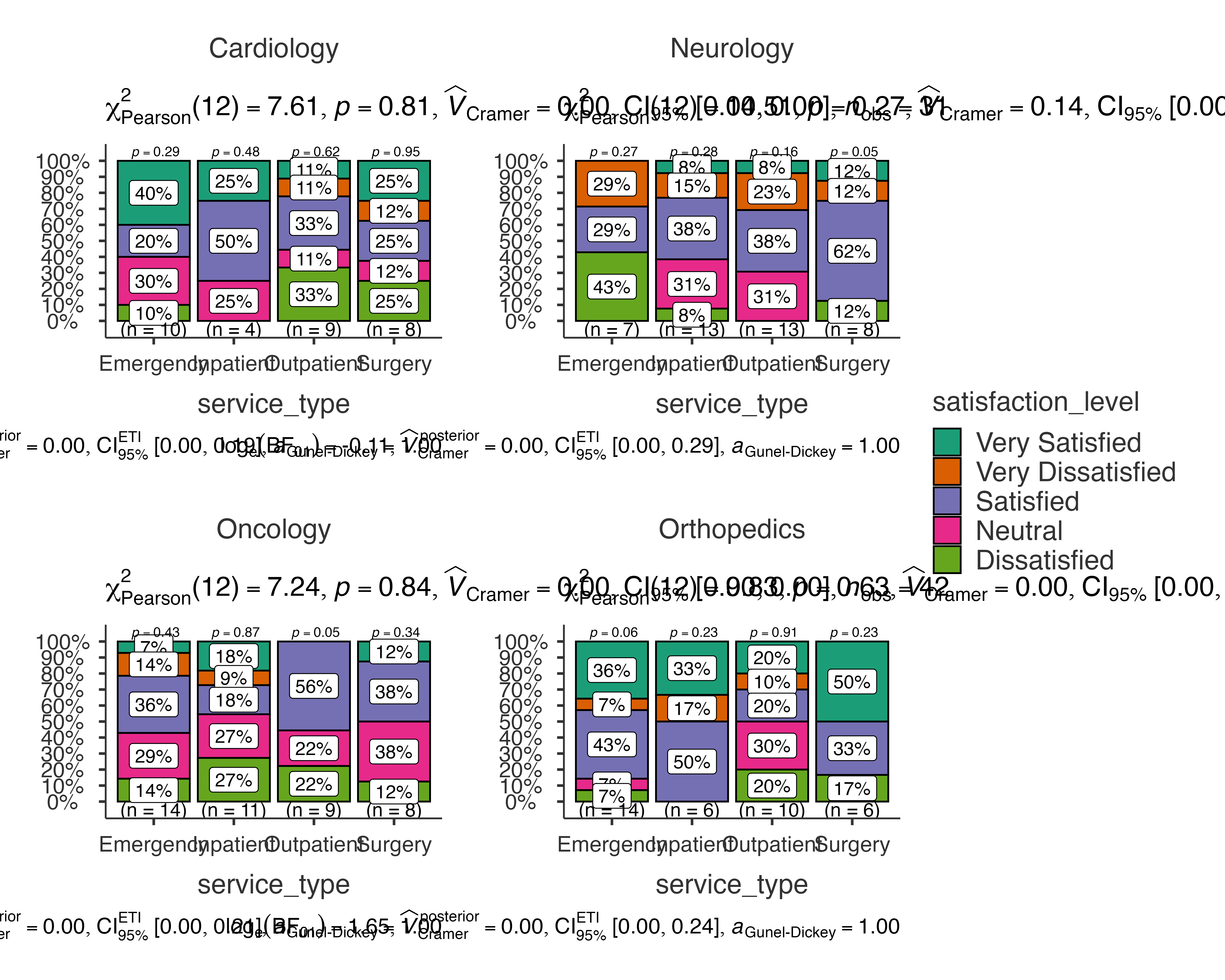

Pairwise Comparisons and Multiple Testing
Enabling Pairwise Comparisons
When you have more than two groups, pairwise comparisons help identify which specific groups differ:
# jjbarstats(
#   data = clinical_trial_data,
#   dep = primary_outcome,
#   group = drug_dosage,
#   pairwisecomparisons = TRUE,
#   padjustmethod = "holm"
# )
Multiple Comparison Correction Methods
Different correction methods are available to control for multiple testing:
# Bonferroni correction (most conservative)
jjbarstats(
  data = diagnostic_test_data,
  dep = test_result,
  group = laboratory,
  pairwisecomparisons = TRUE,
  padjustmethod = "bonferroni"
)
#>
#>  BAR CHARTS
#>
#>  Bar chart analysis comparing test_result by laboratory.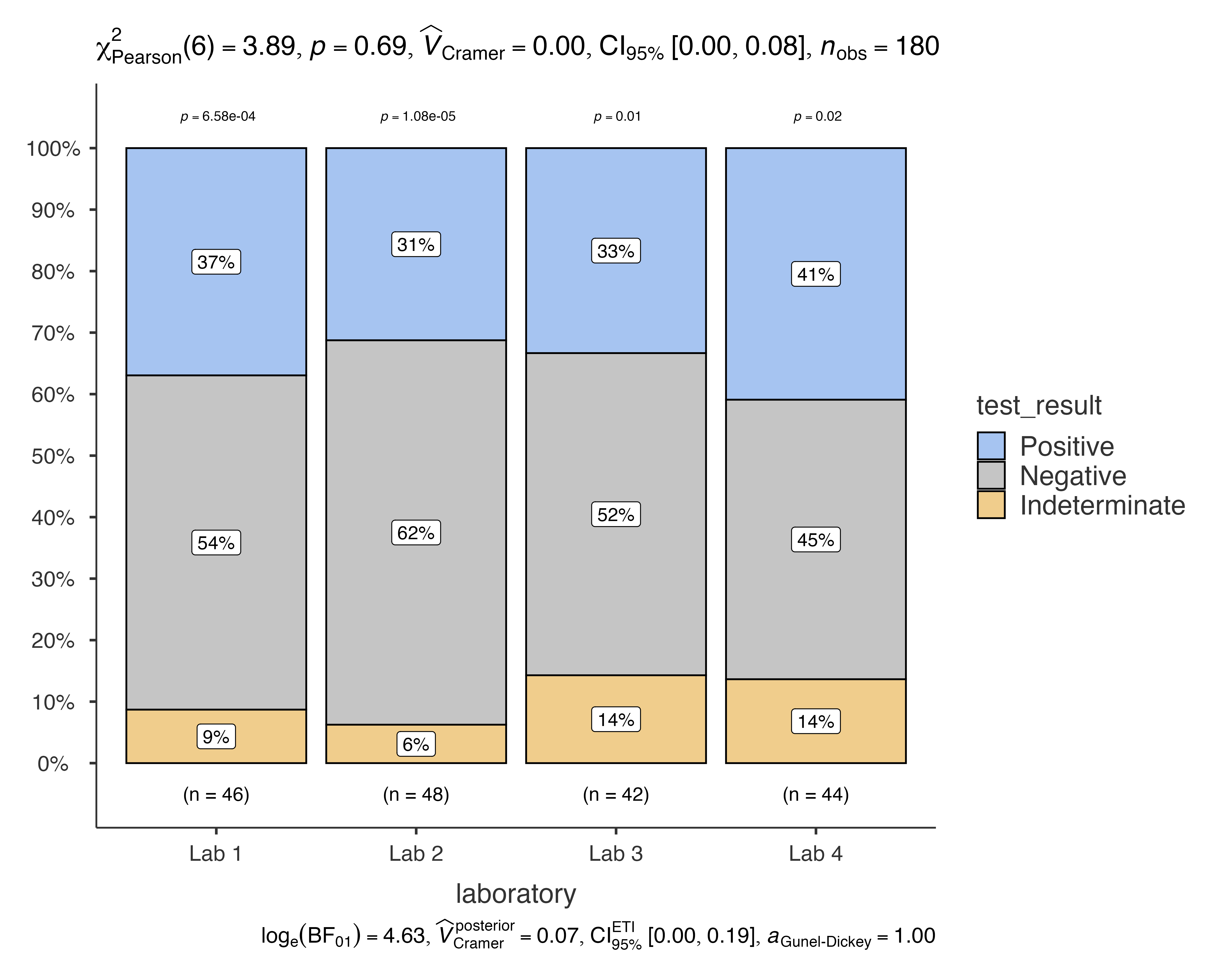
# Benjamini-Hochberg correction (controls false discovery rate)
jjbarstats(
  data = quality_improvement_data,
  dep = priority_level,
  group = department_involved,
  pairwisecomparisons = TRUE,
  padjustmethod = "BH"
)
#>
#>  BAR CHARTS
#>
#>  Bar chart analysis comparing priority_level by department_involved.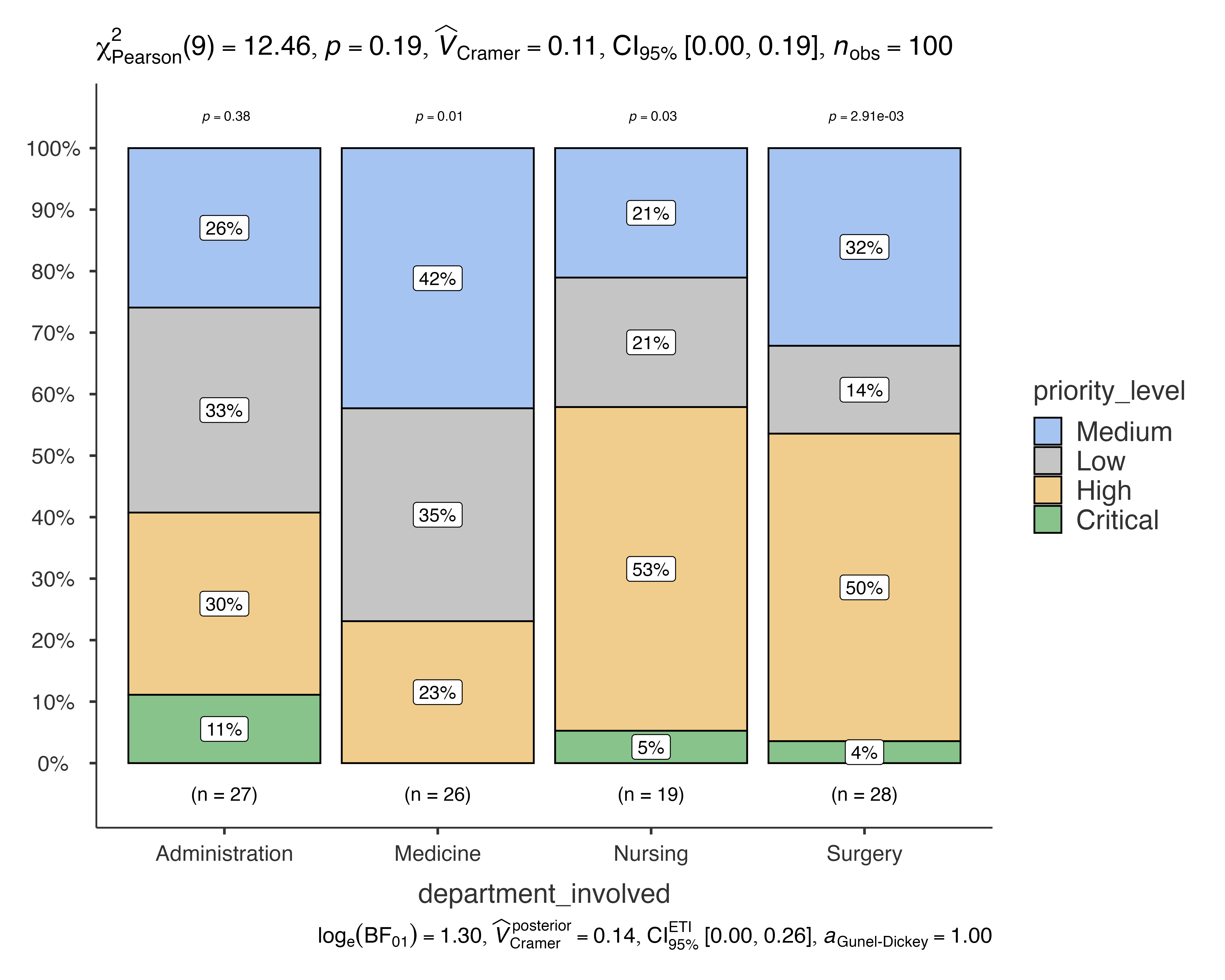
Controlling Pairwise Display
You can control which pairwise comparisons are displayed:
# Show only significant comparisons
jjbarstats(
  data = medical_study_data,
  dep = response,
  group = treatment_group,
  pairwisecomparisons = TRUE,
  pairwisedisplay = "significant"
)
#>
#>  BAR CHARTS
#>
#>  Bar chart analysis comparing response by treatment_group.
# Show all comparisons
jjbarstats(
  data = patient_satisfaction_data,
  dep = staff_rating,
  group = service_type,
  pairwisecomparisons = TRUE,
  pairwisedisplay = "everything"
)
#>
#>  BAR CHARTS
#>
#>  Bar chart analysis comparing staff_rating by service_type.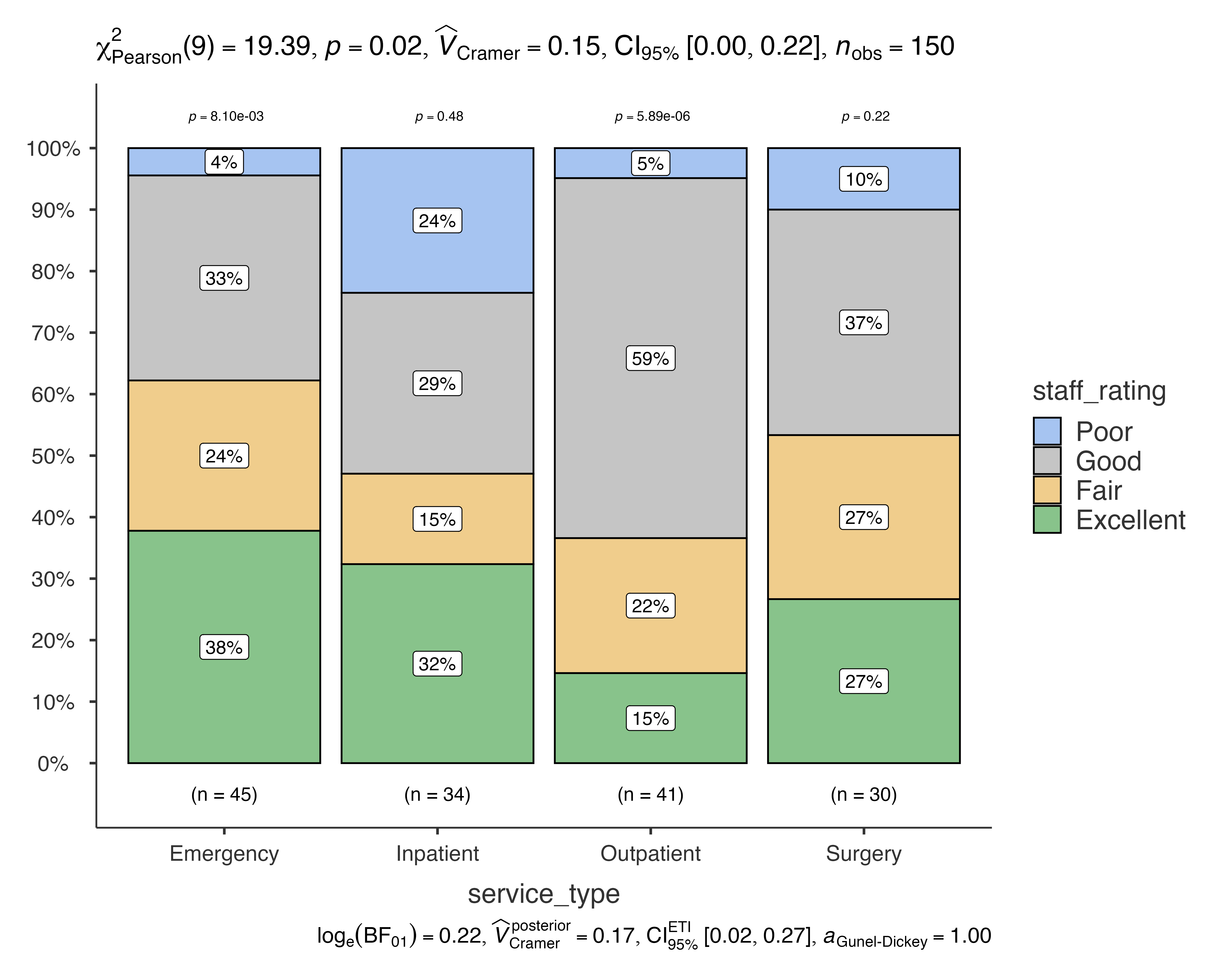
Real-World Clinical Applications
Treatment Efficacy Analysis
Analyzing treatment effectiveness across different patient subgroups:
# Comprehensive treatment analysis
jjbarstats(
  data = medical_study_data,
  dep = response,
  group = treatment_group,
  grvar = severity,
  typestatistics = "nonparametric",
  pairwisecomparisons = TRUE,
  padjustmethod = "BH"
)
#>
#>  BAR CHARTS
#>
#>  Bar chart analysis comparing response by treatment_group, grouped by
#>  severity.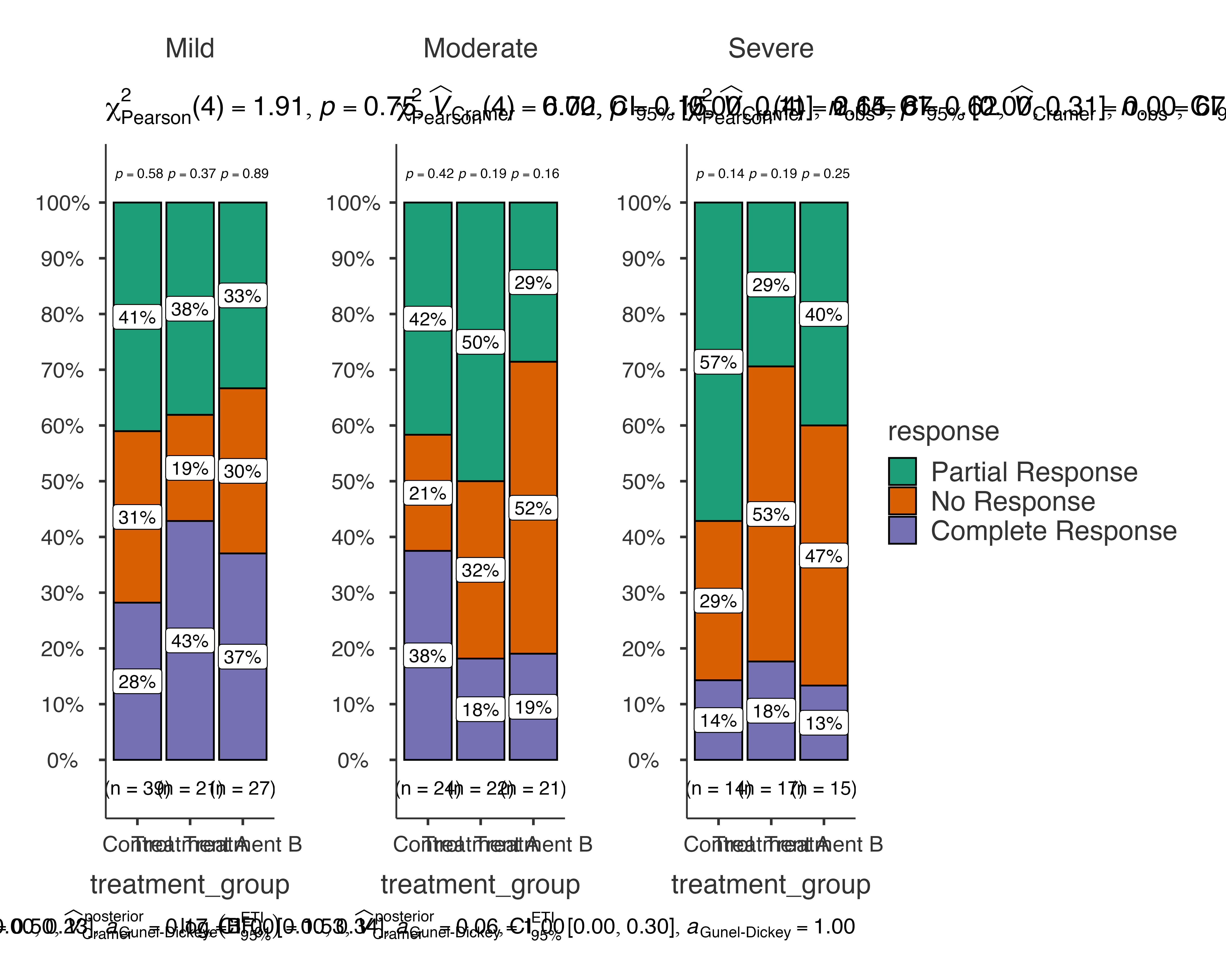

Quality Improvement Analysis
Tracking implementation status across different improvement categories:
jjbarstats(
  data = quality_improvement_data,
  dep = c(implementation_status, priority_level),
  group = improvement_category,
  typestatistics = "parametric",
  pairwisecomparisons = TRUE
)
#>
#>  BAR CHARTS
#>
#>  Bar chart analysis comparing implementation_status, priority_level by
#>  improvement_category.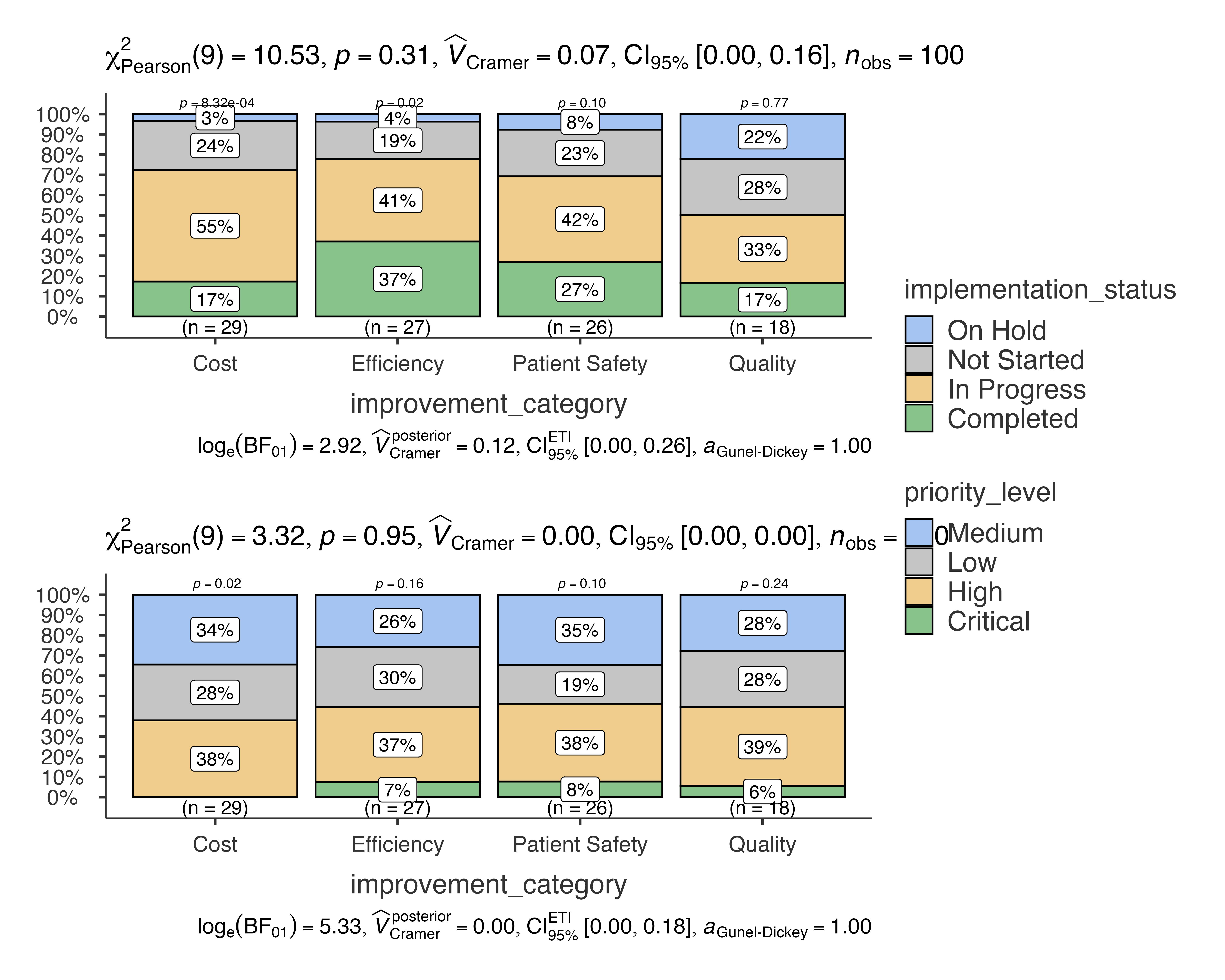
Diagnostic Test Evaluation
Comparing test performance across different methods and laboratories:
jjbarstats(
  data = diagnostic_test_data,
  dep = test_result,
  group = test_method,
  grvar = laboratory,
  typestatistics = "robust",
  pairwisecomparisons = TRUE,
  pairwisedisplay = "significant"
)
#>
#>  BAR CHARTS
#>
#>  Bar chart analysis comparing test_result by test_method, grouped by
#>  laboratory.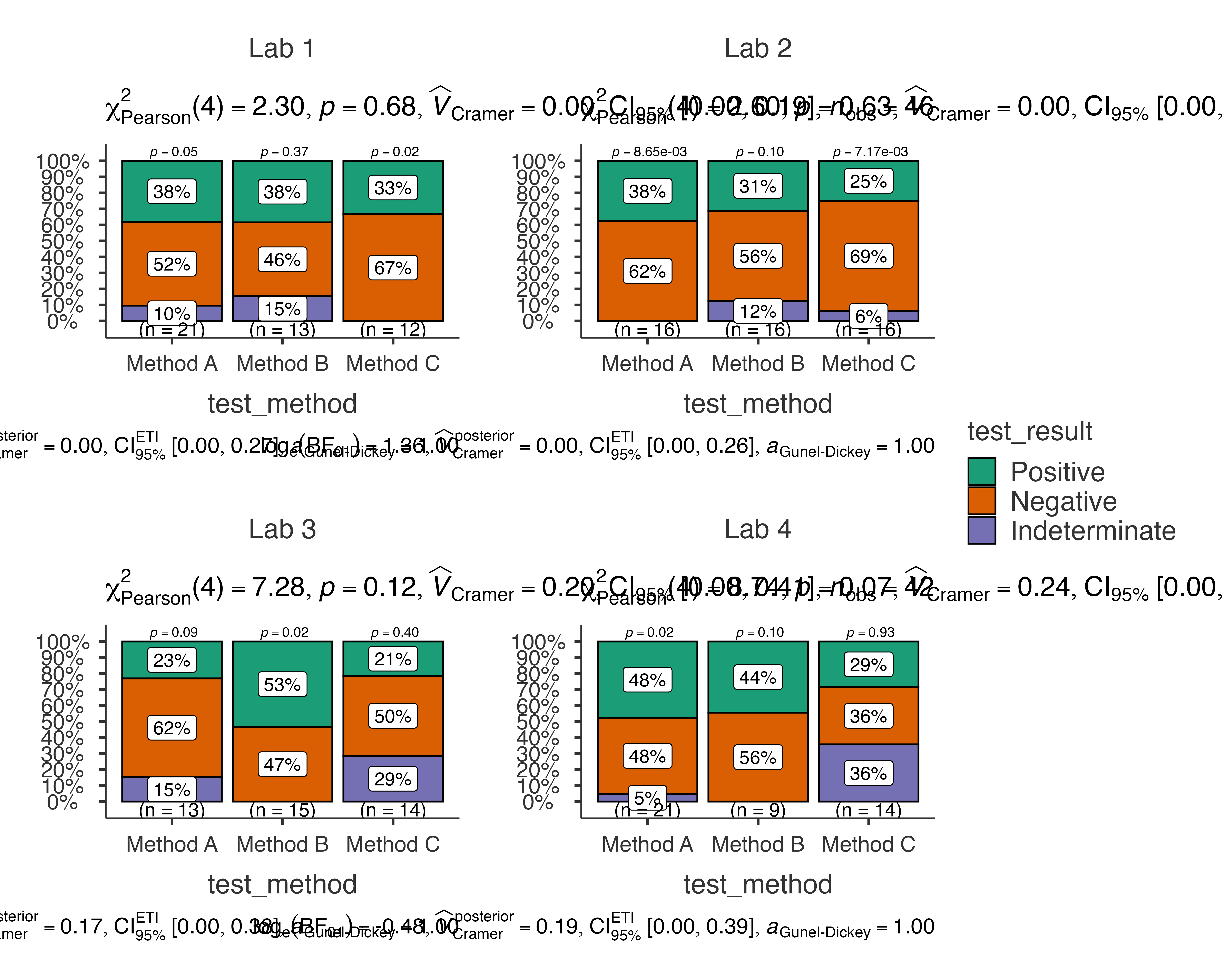

Patient Satisfaction Survey Analysis
Analyzing satisfaction levels across different service types and departments:
jjbarstats(
  data = patient_satisfaction_data,
  dep = satisfaction_level,
  group = service_type,
  grvar = department,
  typestatistics = "nonparametric",
  pairwisecomparisons = TRUE,
  padjustmethod = "holm"
)
#>
#>  BAR CHARTS
#>
#>  Bar chart analysis comparing satisfaction_level by service_type,
#>  grouped by department.

Working with Real Histopathology Data
Using the histopathology dataset that comes with ClinicoPath:
# Analyze lymphovascular invasion by treatment group
jjbarstats(
  data = histopathology,
  dep = LVI,
  group = Group,
  typestatistics = "nonparametric",
  pairwisecomparisons = TRUE
)
#>
#>  BAR CHARTS
#>
#>  Bar chart analysis comparing LVI by Group.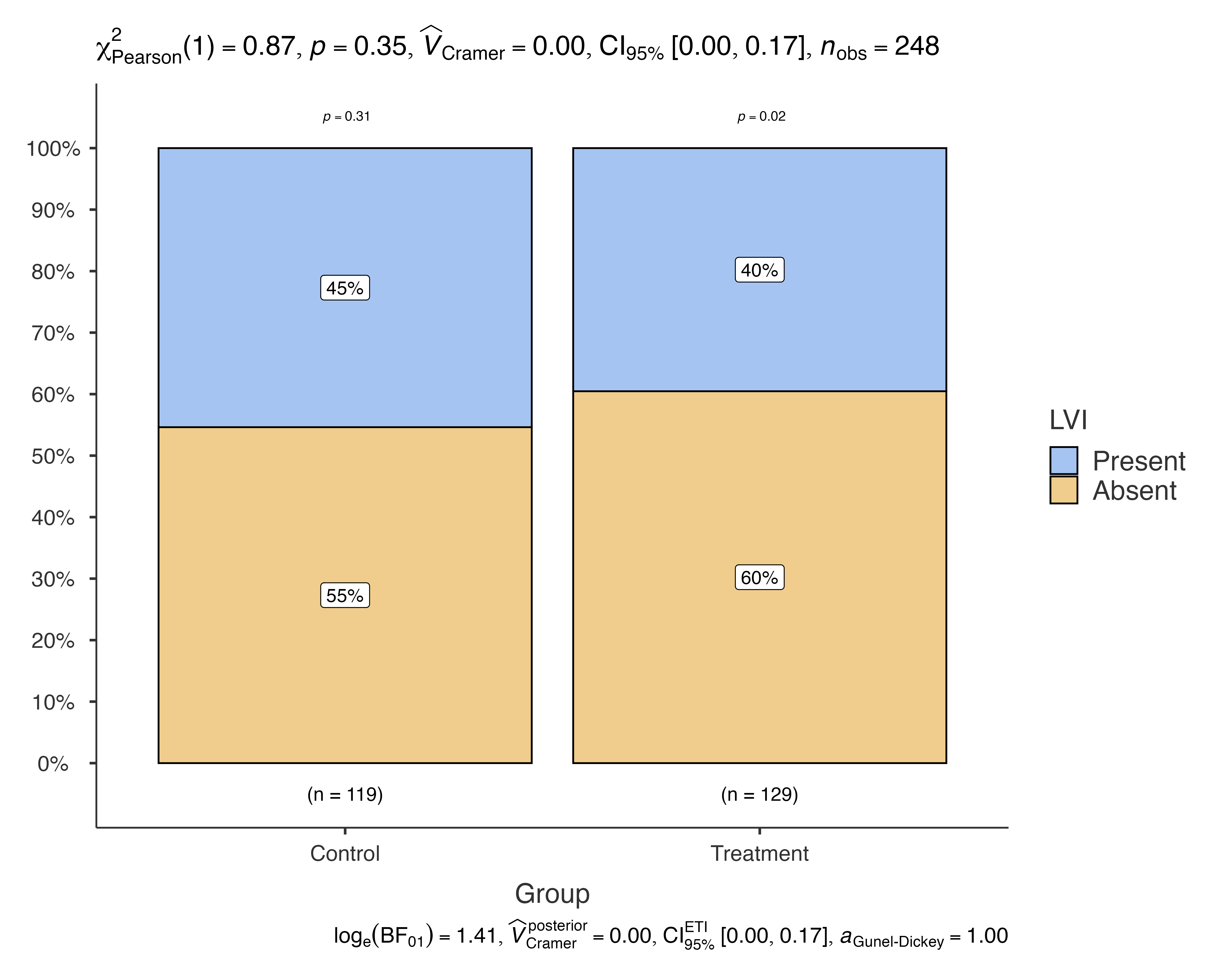
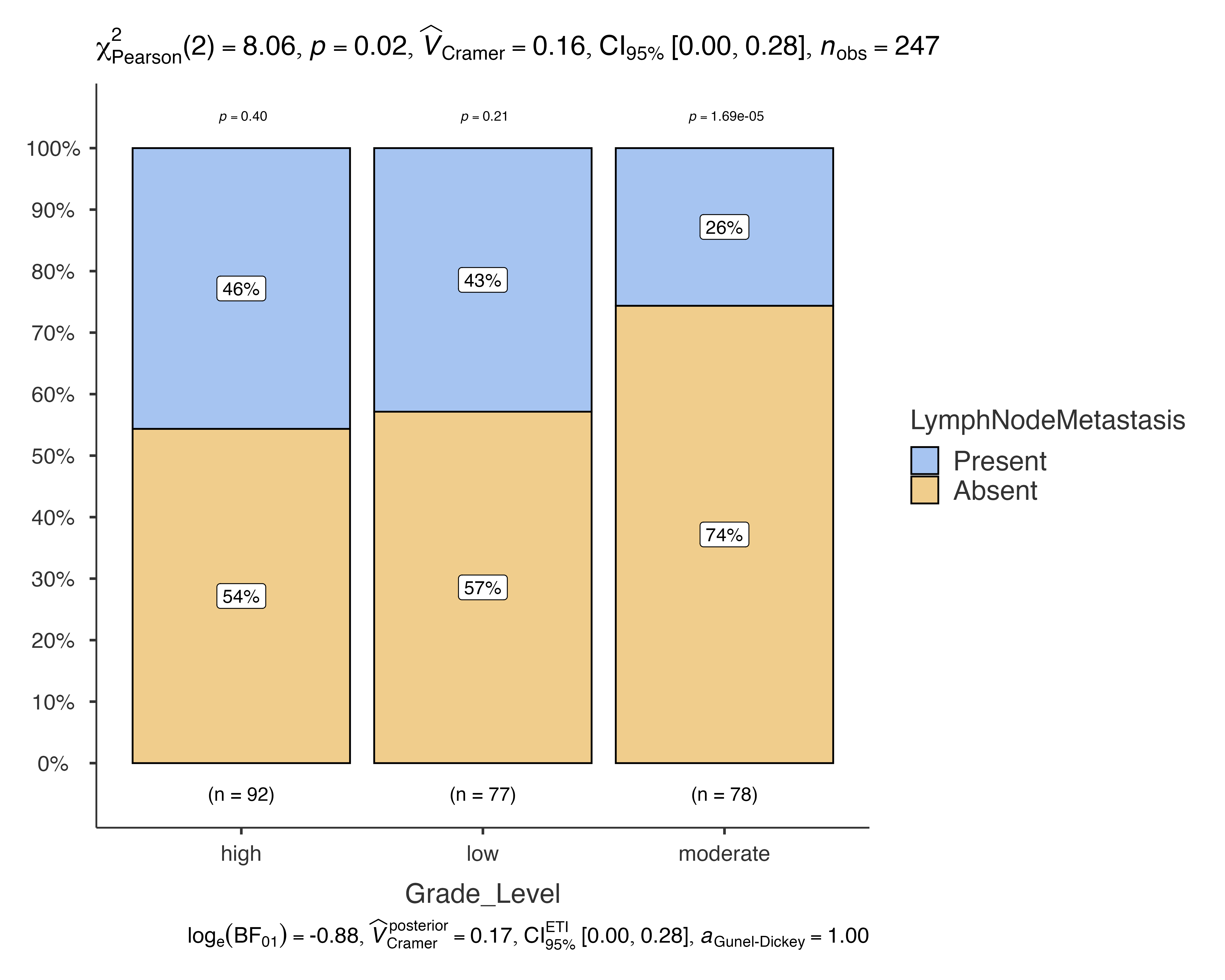
# Multiple outcome analysis
jjbarstats(
  data = histopathology,
  dep = c(LVI, PNI),
  group = Grade_Level,
  typestatistics = "parametric"
)
#>
#>  BAR CHARTS
#>
#>  Bar chart analysis comparing LVI, PNI by Grade_Level.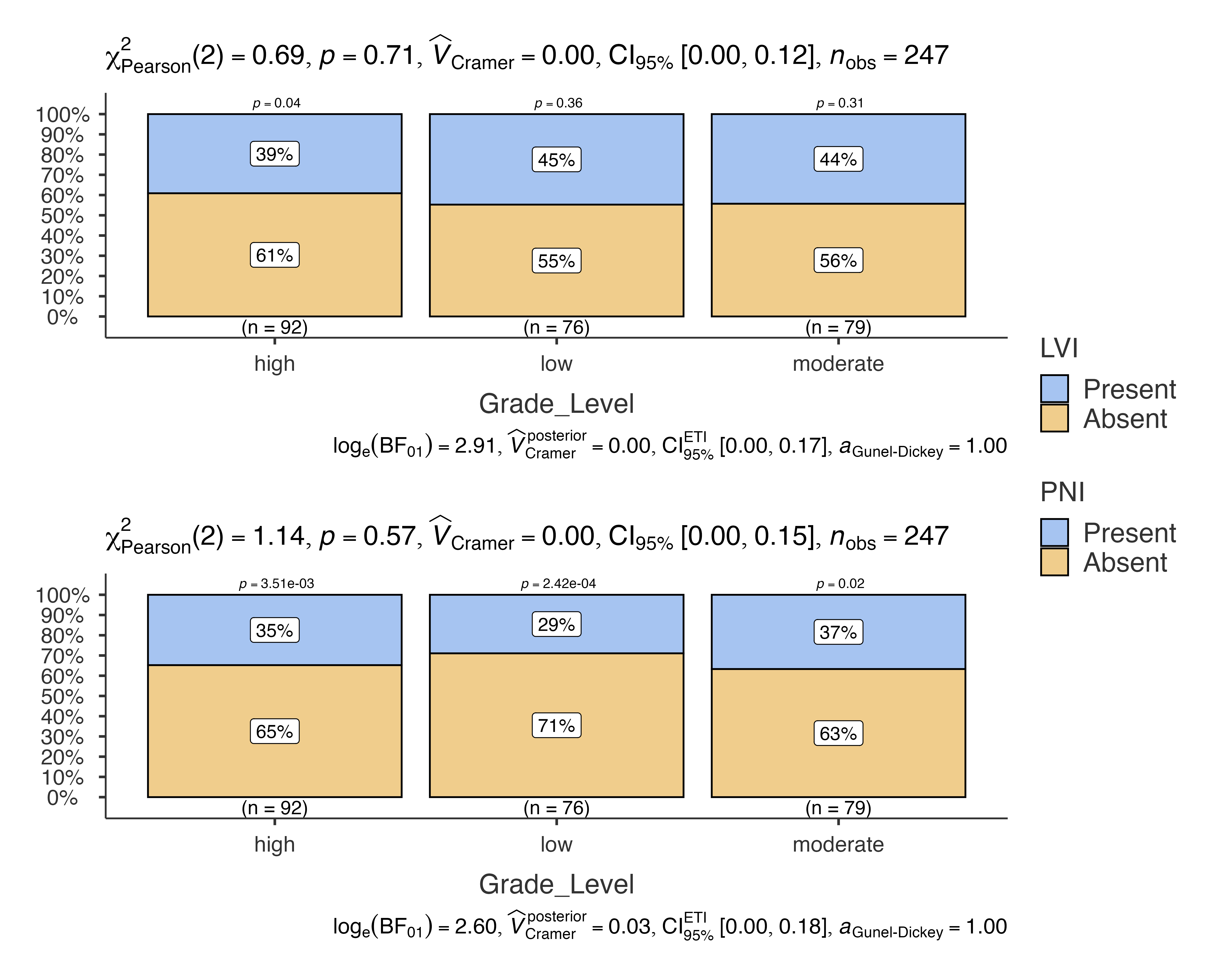
# Grouped analysis by sex
jjbarstats(
  data = histopathology,
  dep = LymphNodeMetastasis,
  group = Grade_Level,
  grvar = Sex,
  typestatistics = "robust",
  pairwisecomparisons = TRUE
)
#>
#>  BAR CHARTS
#>
#>  Bar chart analysis comparing LymphNodeMetastasis by Grade_Level,
#>  grouped by Sex.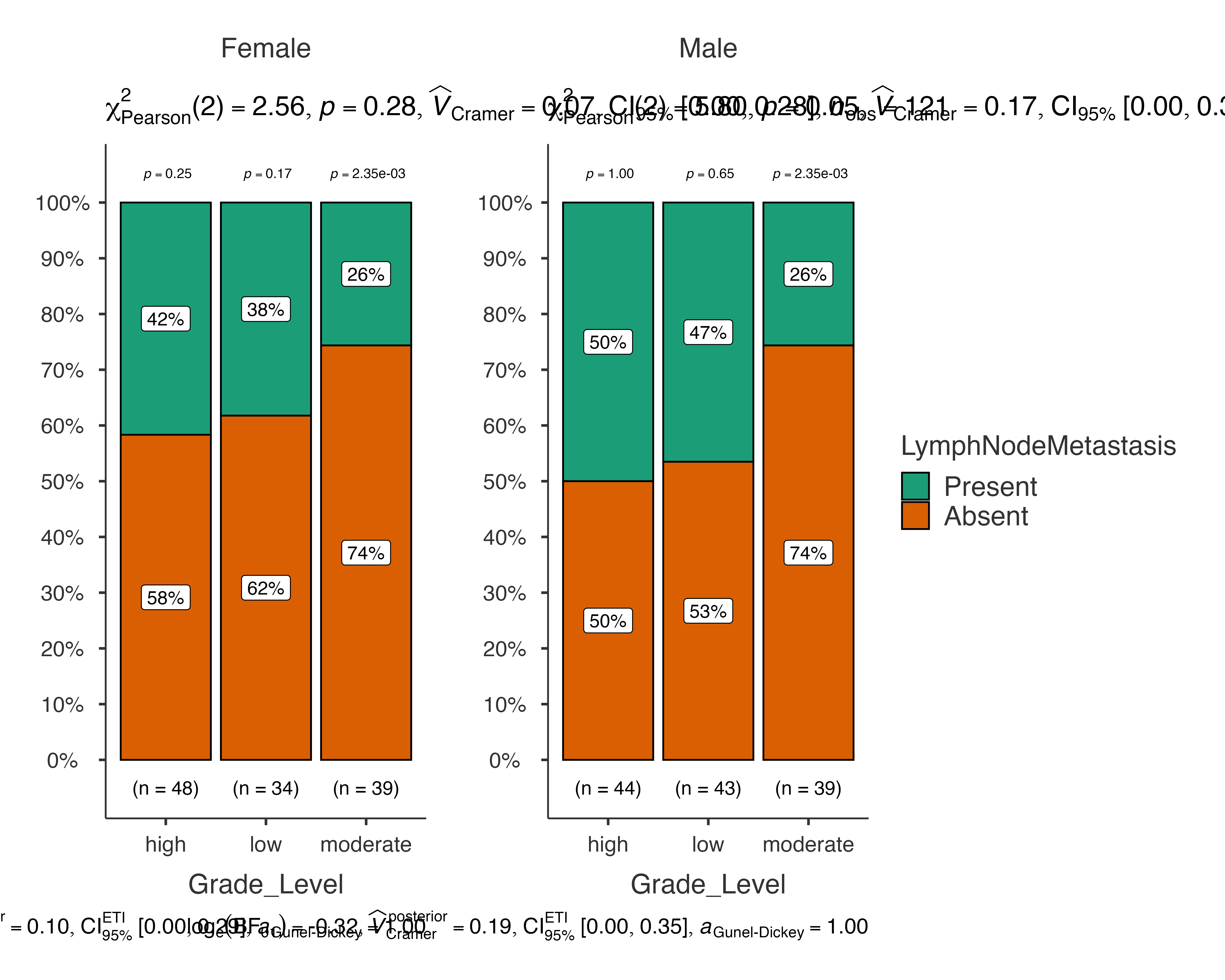
Customization and Theming
Using Original ggstatsplot Theme
jjbarstats(
  data = medical_study_data,
  dep = response,
  group = treatment_group,
  originaltheme = TRUE
)
#>
#>  BAR CHARTS
#>
#>  Bar chart analysis comparing response by treatment_group.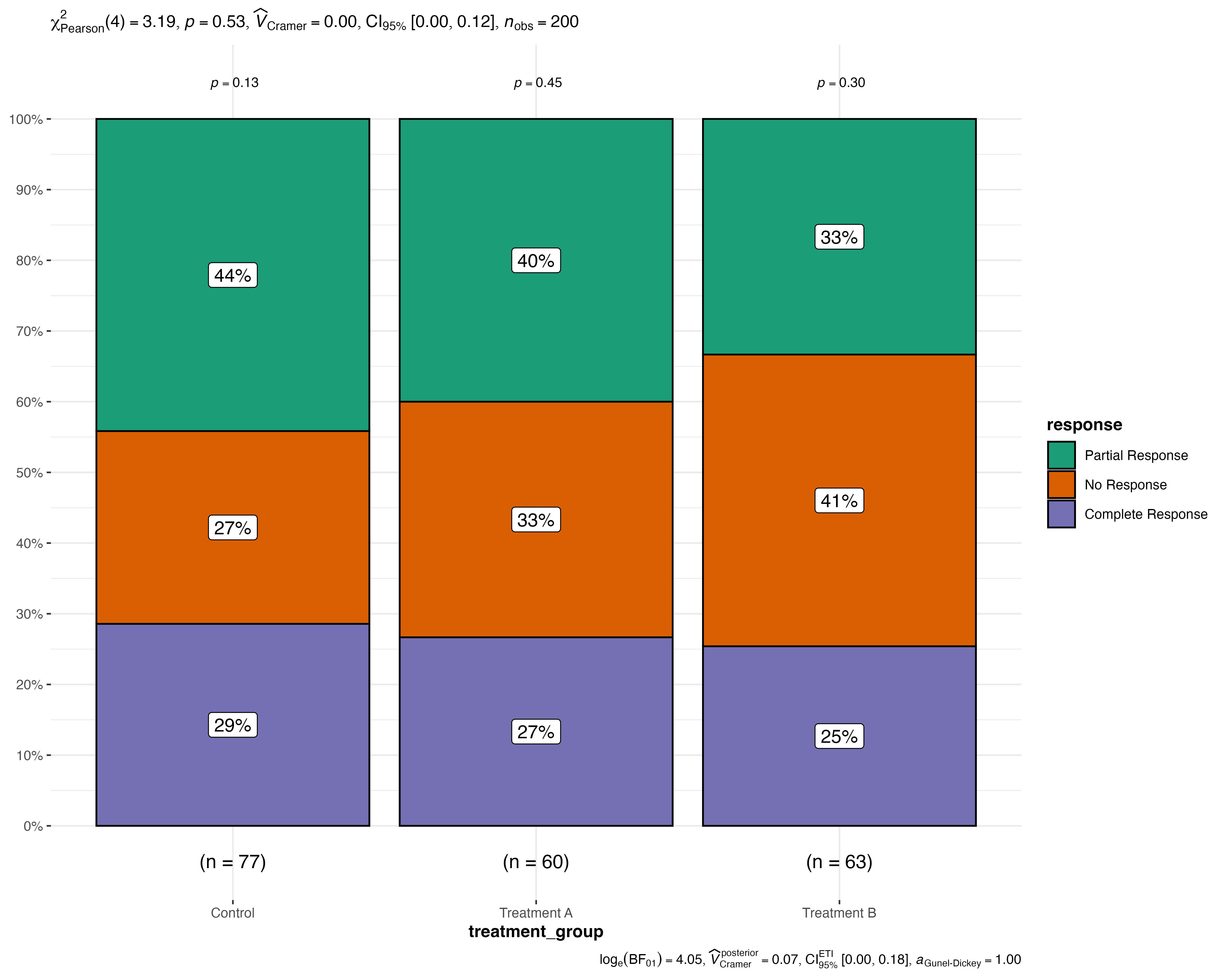
Best Practices and Recommendations
Statistical Method Selection
- Parametric: Use when data meets assumptions (large sample sizes, expected frequencies ≥ 5)
- Non-parametric: Default choice for categorical data, fewer assumptions
- Robust: Good middle ground, less sensitive to outliers
- Bayesian: When you want to incorporate prior knowledge or report Bayes factors
Multiple Comparison Correction
- Holm: Good balance between power and Type I error control
- Bonferroni: Most conservative, use when Type I error is critical
- BH (Benjamini-Hochberg): Controls false discovery rate, good for exploratory analysis
- None: Only when you have specific a priori hypotheses
Sample Size Considerations
- Chi-squared tests require expected frequencies ≥ 5 in each cell
- Fisher’s exact test is automatically used for small samples
- Consider effect sizes, not just p-values
Data Preparation Tips
# Ensure categorical variables are properly formatted
medical_study_clean <- medical_study_data %>%
  mutate(
    treatment_group = factor(treatment_group,
                           levels = c("Control", "Treatment A", "Treatment B")),
    response = factor(response,
                     levels = c("No Response", "Partial Response", "Complete Response"))
  )

# Verify factor levels
str(medical_study_clean[c("treatment_group", "response")])
#> 'data.frame':    200 obs. of  2 variables:
#>  $ treatment_group: Factor w/ 3 levels "Control","Treatment A",..: 2 2 1 3 3 1 1 1 1 3 ...
#>  $ response       : Factor w/ 3 levels "No Response",..: 1 1 1 2 1 3 2 1 3 1 ...
Troubleshooting Common Issues
Issue 1: Empty Cells or Small Counts
When you have empty cells or very small counts, the function automatically switches to appropriate tests:
# Create data with small counts
small_sample <- medical_study_data[1:20, ]

jjbarstats(
  data = small_sample,
  dep = response,
  group = treatment_group,
  typestatistics = "nonparametric"
)
#>
#>  BAR CHARTS
#>
#>  Bar chart analysis comparing response by treatment_group.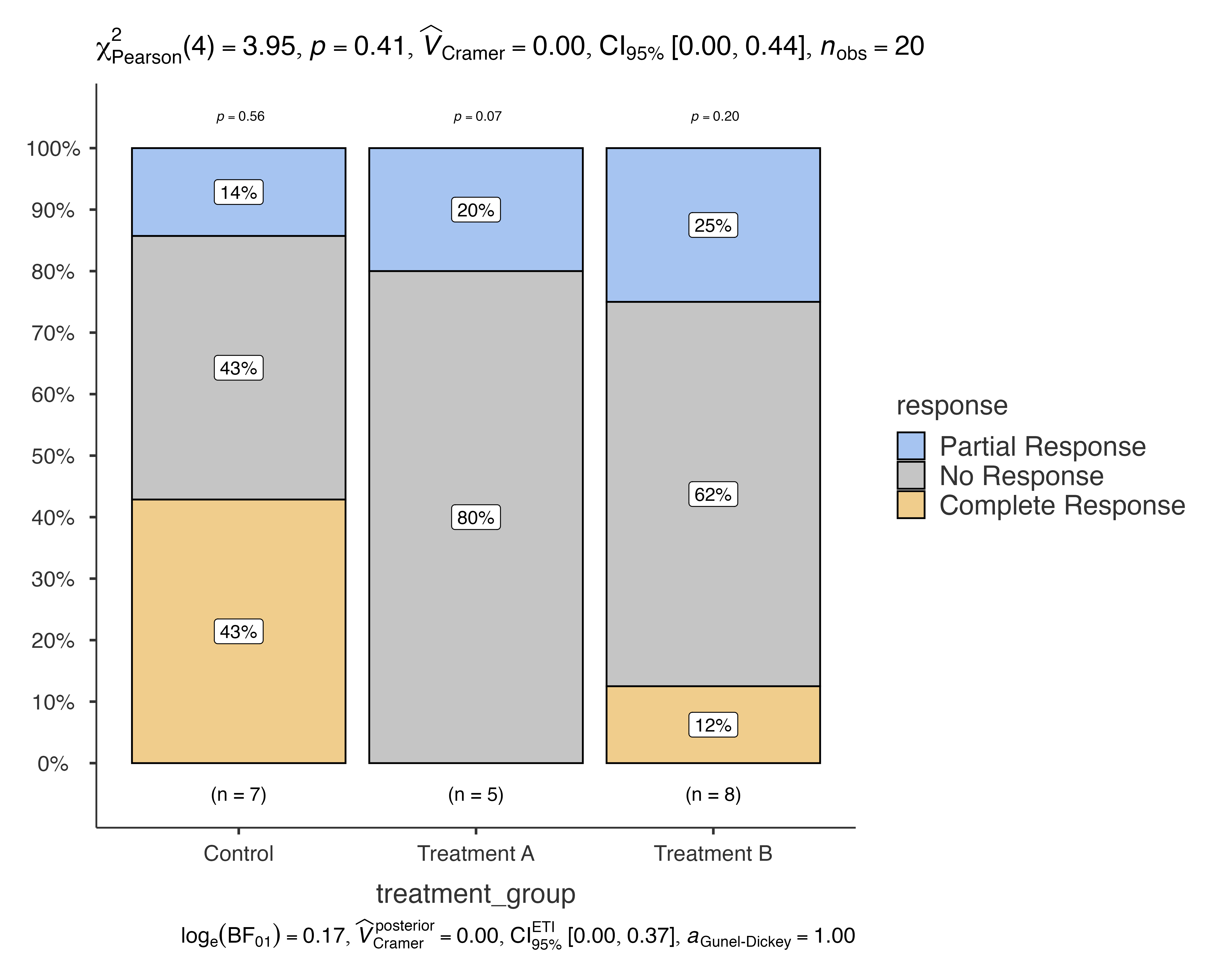
Issue 2: Too Many Categories
When you have many categories, consider grouping or using different visualization:
# Example with multiple categories
jjbarstats(
  data = patient_satisfaction_data,
  dep = satisfaction_level,
  group = department,
  pairwisecomparisons = FALSE  # Disable pairwise for clarity
)
#>
#>  BAR CHARTS
#>
#>  Bar chart analysis comparing satisfaction_level by department.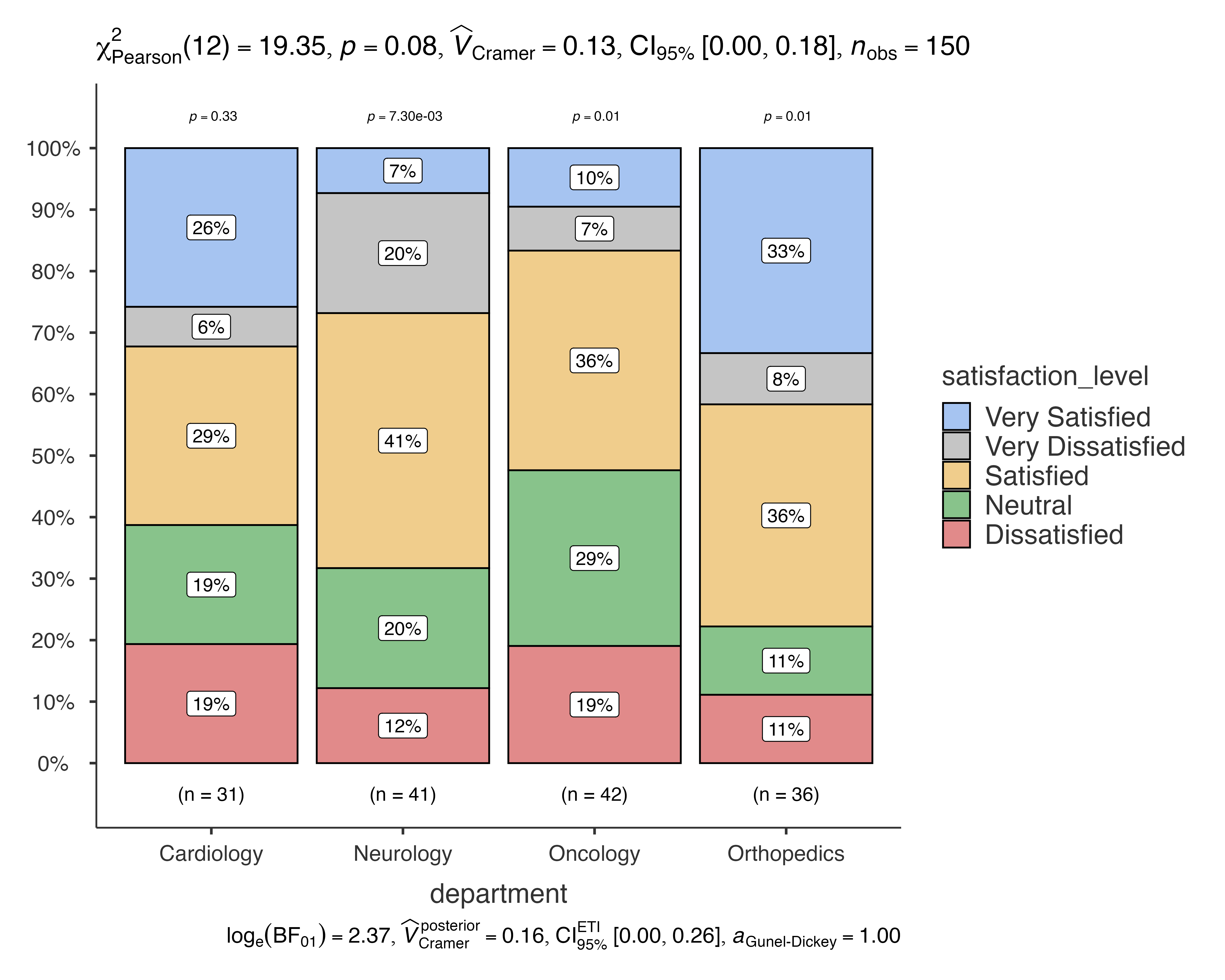
Issue 3: Missing Data
The function automatically handles missing data when
excl = TRUE (default):
# Demonstrate missing data handling
data_with_na <- medical_study_data
data_with_na$response[1:5] <- NA

jjbarstats(
  data = data_with_na,
  dep = response,
  group = treatment_group,
  excl = TRUE  # Exclude missing values
)
#>
#>  BAR CHARTS
#>
#>  Bar chart analysis comparing response by treatment_group.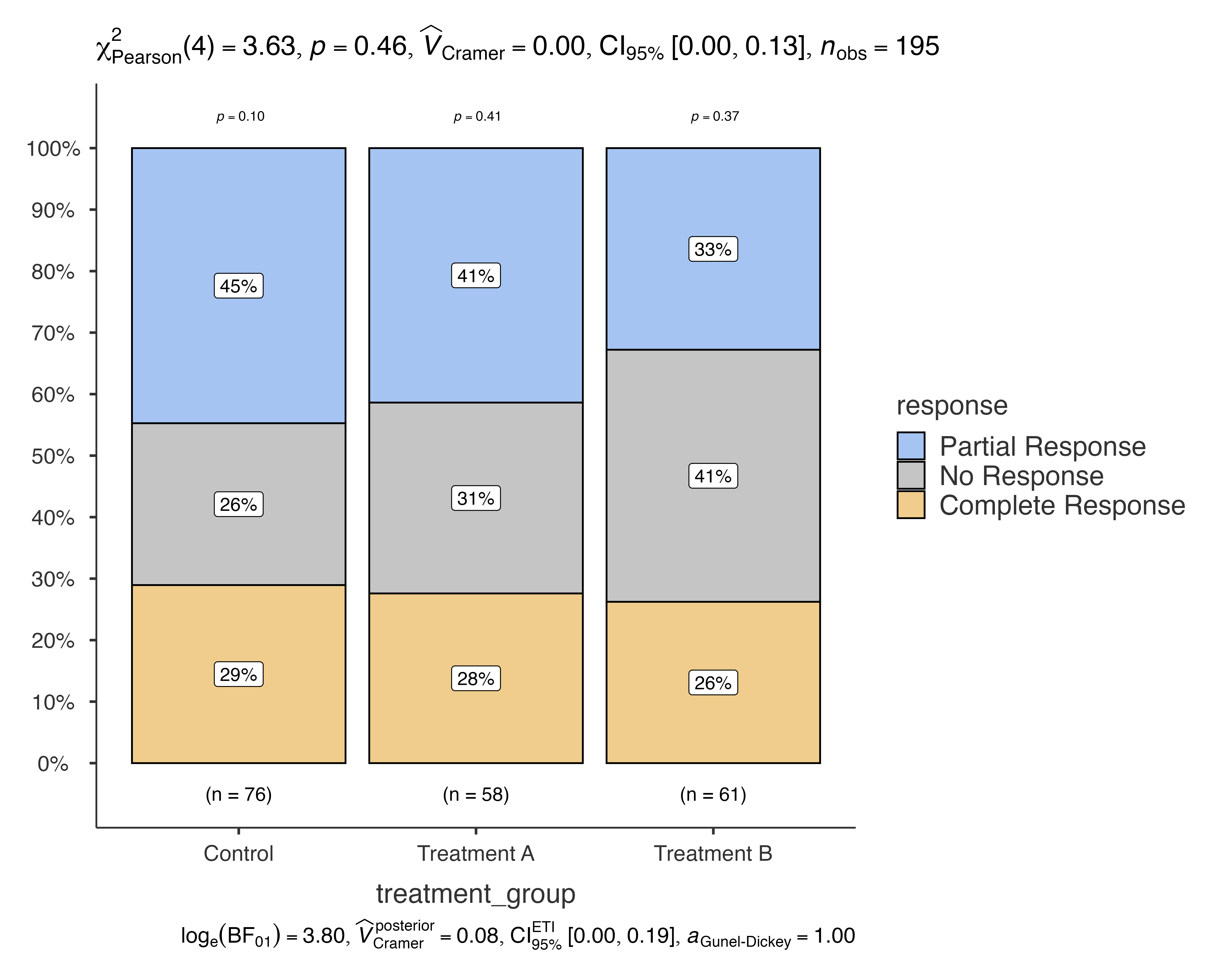
Interpretation Guidelines
Understanding the Statistical Output
- Chi-squared test: Tests independence between categorical variables
- Effect size (Cramér’s V): Measures strength of association (0 = no association, 1 = perfect association)
- Confidence intervals: Provide range of plausible values for the effect
- Pairwise comparisons: Show which specific groups differ
Clinical Significance vs Statistical Significance
- Always consider clinical relevance alongside statistical significance
- Effect sizes help interpret practical importance
- Confidence intervals provide information about precision
Reporting Results
When reporting results from jjbarstats:
- Describe the statistical test used (chi-squared, Fisher’s exact, etc.)
- Report effect size (Cramér’s V) and confidence intervals
- Mention multiple comparison correction if applicable
- Provide sample sizes for each group
- Include the actual plot in your publication
Advanced Examples
Multi-stage Analysis Workflow
# Step 1: Overall analysis
# overall_result <- jjbarstats(
#   data = clinical_trial_data,
#   dep = primary_outcome,
#   group = drug_dosage,
#   typestatistics = "nonparametric",
#   pairwisecomparisons = TRUE,
#   padjustmethod = "BH"
# )

# Step 2: Subgroup analysis by study phase
# subgroup_result <- jjbarstats(
#   data = clinical_trial_data,
#   dep = primary_outcome,
#   group = drug_dosage,
#   grvar = study_phase,
#   typestatistics = "nonparametric",
#   pairwisecomparisons = TRUE
# )Conclusion
The jjbarstats function provides a comprehensive
solution for categorical data analysis in clinical and research
settings. Its integration with the ggstatsplot ecosystem
ensures both statistical rigor and visual appeal, making it an excellent
choice for:
- Clinical trial analysis
- Quality improvement studies
- Survey research
- Diagnostic test evaluation
- Healthcare outcomes research
The function’s flexibility in statistical methods, multiple comparison corrections, and visualization options makes it suitable for both exploratory and confirmatory analysis phases of research projects.
Further Resources
- ggstatsplot documentation
- ClinicoPath package documentation
- Statistical methods references for categorical data analysis
Session Information
sessionInfo()
#> R version 4.5.1 (2025-06-13)
#> Platform: aarch64-apple-darwin20
#> Running under: macOS Sequoia 15.5
#>
#> Matrix products: default
#> BLAS:   /Library/Frameworks/R.framework/Versions/4.5-arm64/Resources/lib/libRblas.0.dylib
#> LAPACK: /Library/Frameworks/R.framework/Versions/4.5-arm64/Resources/lib/libRlapack.dylib;  LAPACK version 3.12.1
#>
#> locale:
#> [1] en_US.UTF-8/en_US.UTF-8/en_US.UTF-8/C/en_US.UTF-8/en_US.UTF-8
#>
#> time zone: Europe/Istanbul
#> tzcode source: internal
#>
#> attached base packages:
#> [1] stats     graphics  grDevices utils     datasets  methods   base
#>
#> other attached packages:
#> [1] dplyr_1.1.4          ggplot2_3.5.2        ClinicoPath_0.0.3.56
#>
#> loaded via a namespace (and not attached):
#>   [1] igraph_2.1.4            plotly_4.11.0           Formula_1.2-5
#>   [4] cutpointr_1.2.1         rematch2_2.1.2          timeROC_0.4
#>   [7] tidyselect_1.2.1        vtree_5.1.9             lattice_0.22-7
#>  [10] stringr_1.5.1           lgr_0.4.4               parallel_4.5.1
#>  [13] caret_7.0-1             dichromat_2.0-0.1       correlation_0.8.8
#>  [16] png_0.1-8               cli_3.6.5               bayestestR_0.16.1
#>  [19] askpass_1.2.1           arsenal_3.6.3           openssl_2.3.3
#>  [22] ggeconodist_0.1.0       countrycode_1.6.1       pkgdown_2.1.3
#>  [25] textshaping_1.0.1       paradox_1.0.1           purrr_1.0.4
#>  [28] officer_0.6.10          naivebayes_1.0.0        stars_0.6-8
#>  [31] broom.mixed_0.2.9.6     ggflowchart_1.0.0       ggoncoplot_0.1.0
#>  [34] curl_6.4.0              strucchange_1.5-4       mime_0.13
#>  [37] evaluate_1.0.4          coin_1.4-3              V8_6.0.4
#>  [40] stringi_1.8.7           pROC_1.18.5             backports_1.5.0
#>  [43] desc_1.4.3              mlr3extralearners_1.0.0 lmerTest_3.1-3
#>  [46] XML_3.99-0.18           Exact_3.3               tinytable_0.10.0
#>  [49] lubridate_1.9.4         httpuv_1.6.16           mlr3viz_0.10.1
#>  [52] paletteer_1.6.0         magrittr_2.0.3          rappdirs_0.3.3
#>  [55] splines_4.5.1           prodlim_2025.04.28      r2rtf_1.1.4
#>  [58] KMsurv_0.1-6            BiasedUrn_2.0.12        survminer_0.5.0
#>  [61] logger_0.4.0            epiR_2.0.84             wk_0.9.4
#>  [64] palmerpenguins_0.1.1    networkD3_0.4.1         finalfit_1.0.8
#>  [67] DT_0.33                 lpSolve_5.6.23          rootSolve_1.8.2.4
#>  [70] DBI_1.2.3               terra_1.8-54            jquerylib_0.1.4
#>  [73] withr_3.0.2             reformulas_0.4.1        class_7.3-23
#>  [76] systemfonts_1.2.3       lmtest_0.9-40           rprojroot_2.0.4
#>  [79] leaflegend_1.2.1        RefManageR_1.4.0        htmlwidgets_1.6.4
#>  [82] fs_1.6.6                waffle_1.0.2            ggvenn_0.1.10
#>  [85] gtsummary_2.3.0         cellranger_1.1.0        summarytools_1.1.4
#>  [88] extrafont_0.19          lmom_3.2                effectsize_1.0.1
#>  [91] zoo_1.8-14              raster_3.6-32           knitr_1.50
#>  [94] ggcharts_0.2.1          gt_1.0.0                timechange_0.3.0
#>  [97] foreach_1.5.2           dcurves_0.5.0           patchwork_1.3.1
#> [100] visNetwork_2.1.2        grid_4.5.1              data.table_1.17.8
#> [103] timeDate_4041.110       gsDesign_3.6.9          pan_1.9
#> [106] quantreg_6.1            psych_2.5.6             extrafontdb_1.0
#> [109] DiagrammeR_1.0.11       clintools_0.9.10.1      DescTools_0.99.60
#> [112] lazyeval_0.2.2          yaml_2.3.10             leaflet_2.2.2
#> [115] easyalluvial_0.3.2      useful_1.2.6.1          survival_3.8-3
#> [118] crosstable_0.8.1        lwgeom_0.2-14           crayon_1.5.3
#> [121] RColorBrewer_1.1-3      tidyr_1.3.1             progressr_0.15.1
#> [124] tweenr_2.0.3            later_1.4.2             jtools_2.3.0
#> [127] microbenchmark_1.5.0    ggridges_0.5.6          mlr3measures_1.0.0
#> [130] codetools_0.2-20        base64enc_0.1-3         labelled_2.14.1
#> [133] shape_1.4.6.1           estimability_1.5.1      gdtools_0.4.2
#> [136] data.tree_1.1.0         foreign_0.8-90          pkgconfig_2.0.3
#> [139] grafify_5.0.0.1         xml2_1.3.8              ggpubr_0.6.1
#> [142] performance_0.15.0      viridisLite_0.4.2       xtable_1.8-4
#> [145] bibtex_0.5.1            car_3.1-3               plyr_1.8.9
#> [148] httr_1.4.7              rbibutils_2.3           tools_4.5.1
#> [151] globals_0.18.0          hardhat_1.4.1           cols4all_0.8
#> [154] htmlTable_2.4.3         broom_1.0.8             checkmate_2.3.2
#> [157] nlme_3.1-168            MatrixModels_0.5-4      regions_0.1.8
#> [160] survMisc_0.5.6          maptiles_0.10.0         crosstalk_1.2.1
#> [163] assertthat_0.2.1        lme4_1.1-37             digest_0.6.37
#> [166] numDeriv_2016.8-1.1     Matrix_1.7-3            tmap_4.1
#> [169] furrr_0.3.1             farver_2.1.2            tzdb_0.5.0
#> [172] reshape2_1.4.4          viridis_0.6.5           pec_2023.04.12
#> [175] rapportools_1.2         gghalves_0.1.4          ModelMetrics_1.2.2.2
#> [178] crul_1.5.0              rpart_4.1.24            glue_1.8.0
#> [181] mice_3.18.0             cachem_1.1.0            ggswim_0.1.0
#> [184] polyclip_1.10-7         UpSetR_1.4.0            Hmisc_5.2-3
#> [187] generics_0.1.4          visdat_0.6.0            classInt_0.4-11
#> [190] stats4_4.5.1            ggalluvial_0.12.5       mvtnorm_1.3-3
#> [193] survey_4.4-2            powerSurvEpi_0.1.5      ggfortify_0.4.18
#> [196] parallelly_1.45.0       ISOweek_0.6-2           mnormt_2.1.1
#> [199] ggmice_0.1.0            here_1.0.1              ragg_1.4.0
#> [202] pbapply_1.7-2           fontBitstreamVera_0.1.1 carData_3.0-5
#> [205] minqa_1.2.8             httr2_1.1.2             giscoR_0.6.1
#> [208] tcltk_4.5.1             rpart.plot_3.1.2        coefplot_1.2.8
#> [211] eurostat_4.0.0          glmnet_4.1-9            jmvcore_2.6.3
#> [214] spacesXYZ_1.6-0         gower_1.0.2             mitools_2.4
#> [217] readxl_1.4.5            datawizard_1.1.0        httpcode_0.3.0
#> [220] fontawesome_0.5.3       ggsignif_0.6.4          timereg_2.0.6
#> [223] party_1.3-18            gridExtra_2.3           shiny_1.11.1
#> [226] lava_1.8.1              tmaptools_3.2           parameters_0.27.0
#> [229] arcdiagram_0.1.12       rmarkdown_2.29          TidyDensity_1.5.0
#> [232] pander_0.6.6            mlr3misc_0.18.0         scales_1.4.0
#> [235] gld_2.6.7               svglite_2.2.1           future_1.58.0
#> [238] fontLiberation_0.1.0    DiagrammeRsvg_0.1       ggpp_0.5.9
#> [241] km.ci_0.5-6             rstudioapi_0.17.1       janitor_2.2.1
#> [244] cluster_2.1.8.1         rstantools_2.4.0        hms_1.1.3
#> [247] anytime_0.3.11          colorspace_2.1-1        rlang_1.1.6
#> [250] jomo_2.7-6              s2_1.1.9                pivottabler_1.5.6
#> [253] ipred_0.9-15            ggforce_0.5.0           kknn_1.4.1
#> [256] mgcv_1.9-3              xfun_0.52               coda_0.19-4.1
#> [259] e1071_1.7-16            TH.data_1.1-3           modeltools_0.2-24
#> [262] matrixStats_1.5.0       benford.analysis_0.1.5  recipes_1.3.1
#> [265] iterators_1.0.14        emmeans_1.11.1          randomForest_4.7-1.2
#> [268] abind_1.4-8             tibble_3.3.0            libcoin_1.0-10
#> [271] ggrain_0.0.4            readr_2.1.5             Rdpack_2.6.4
#> [274] promises_1.3.3          sandwich_3.1-1          proxy_0.4-27
#> [277] compiler_4.5.1          statsExpressions_1.7.0  forcats_1.0.0
#> [280] leaflet.providers_2.0.0 boot_1.3-31             distributional_0.5.0
#> [283] tableone_0.13.2         SparseM_1.84-2          polynom_1.4-1
#> [286] listenv_0.9.1           Rcpp_1.1.0              Rttf2pt1_1.3.12
#> [289] fontquiver_0.2.1        DataExplorer_0.8.3      datefixR_1.7.0
#> [292] rms_8.0-0               units_0.8-7             MASS_7.3-65
#> [295] uuid_1.2-1              insight_1.3.1           R6_2.6.1
#> [298] fastmap_1.2.0           multcomp_1.4-28         rstatix_0.7.2
#> [301] BayesFactor_0.9.12-4.7  vcd_1.4-13              ggstatsplot_0.13.1
#> [304] mitml_0.4-5             ggdist_3.3.3            nnet_7.3-20
#> [307] gtable_0.3.6            leafem_0.2.4            KernSmooth_2.23-26
#> [310] miniUI_0.1.2            irr_0.84.1              gtExtras_0.6.0
#> [313] htmltools_0.5.8.1       tidyplots_0.3.1.9000    leafsync_0.1.0
#> [316] RcppParallel_5.1.10     polspline_1.1.25        lifecycle_1.0.4
#> [319] sf_1.0-21               zip_2.3.3               kableExtra_1.4.0
#> [322] pryr_0.1.6              nloptr_2.2.1            mlr3_1.0.1
#> [325] mlr3learners_0.12.0     sass_0.4.10             vctrs_0.6.5
#> [328] zeallot_0.2.0           snakecase_0.11.1        flextable_0.9.9
#> [331] rcrossref_1.2.0         haven_2.5.5             sp_2.2-0
#> [334] pracma_2.4.4            future.apply_1.20.0     bslib_0.9.0
#> [337] pillar_1.11.0           prismatic_1.1.2         magick_2.8.7
#> [340] moments_0.14.1          jsonlite_2.0.0          expm_1.0-0